The mode is the value that occurs most frequently in the data. Spreadsheet programs such as Microsoft Excel or OpenOffice.org Calc can determine the mode with the function MODE.
=MODE(data)
In the Fall of 2000 the statistics class gathered data on the number of siblings for each member of the class. One student was an only child and had no siblings. One student had 13 brothers and sisters. The complete data set is as follows:
1,2,2,2,2,2,3,3,4,4,4,5,5,5,7,8,9,10,12,12,13
The mode is 2 because 2 occurs more often than any other value. Where there is a tie there is no mode.
For the ages of students in that class
18,19,19,20,20,21,21,21,21,22,22,22,22,23,23,24,24,25,25,26
...there is no mode: there is a tie between 21 and 22, hence there no single must frequent value. Spreadsheets will, however, usually report a mode of 21 in this case. Spreadsheets often select the first mode in a multi-modal tie.
If all values appear only once, then there is no mode. Spreadsheets will display #N/A or #VALUE to indicate an error has occurred - there is no mode. No mode is NOT the same as a mode of zero. A mode of zero means that zero is the most frequent data value. Do not put the number 0 (zero) for "no mode." An example of a mode of zero might be the number of children for students in statistics class.
The median is the central (or middle) value in a data set. If a number sits at the middle, then it is the median. If the middle is between two numbers, then the median is half way between the two middle numbers.
For the sibling data...
1,2,2,2,2,2,3,3,4,4,|4|,5,5,5,7,8,9,10,12,12,13
...the median is 4.
Note the data must be in order (sorted) before you can find the median. For the data 2, 4, 6, 8 the median is 5: (4+6)/2.
The median function in spreadsheets is MEDIAN.
=MEDIAN(data)
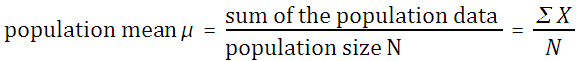
The mean, also called the arithmetic mean and also called the average, is calculated mathematically by adding the values and then dividing by the number of values (the sample size n).
If the mean is the mean of a population, then it is called the population mean μ. The letter μ is a Greek lower case "m" and is pronounced "mu."
If the mean is the mean of a sample, then it is the sample mean x. The symbol x is pronounced "x bar."
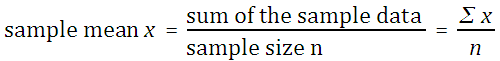
The sum of the data ∑ x can be determined using the function =SUM(data). The sample size n can be determined using =COUNT(data). Thus =SUM(data)/COUNT(data) will calculate the mean. There is also a single function that calculates the mean. The function that directly calculates the mean is AVERAGE
=AVERAGE(data)
Resistant measures: One that is not influenced by extremely high or extremely low data values. The median tends to be more resistant than mean.
If the mean is measured using the whole population then this would be the population mean. If the mean was calculated from a sample then the mean is the sample mean. Mathematically there is no difference in the way the population and sample mean are calculated.
The midrange is the midway point between the minimum and the maximum in a set of data. The midrange is calculated from:
midrange = (maximum + minimum)/2
In a spreadsheet use the following formula:
=(MAX(data)+MIN(data))/2
Consider the following data:
| Data | mode | median | mean μ | min | max | range | midrange | |
|---|---|---|---|---|---|---|---|---|
| Data set 1 | 5, 5, 5, 5 | 5 | 5 | 5 | 5 | 5 | 0 | 0 |
| Data set 2 | 2, 4, 6, 8 | none | 5 | 5 | 2 | 8 | 6 | 5 |
| Data set 3 | 2, 2, 8, 8 | none | 5 | 5 | 2 | 8 | 6 | 5 |
Neither the mode, median, nor the mean reveal clearly the differences in the distribution of the data above. The mean and the median are the same for each data set. The mode is the same as the mean and the median for the first data set and is unavailable for the last data set (spreadsheets will report a mode of 2 for the last data set). A single number that would characterize how much the data is spread out would be useful.
The range is one way to capture the spread of the data. The range is calculated by subtracting the smallest value from the largest value. In a spreadsheet:
=MAX(data) − MIN(data)
The range still does not characterize the difference between set 2 and 3: the last set has more data further away from the center of the data distribution. The range misses this difference.
To capture the spread of the data we use a measure related to the average distance of the data from the mean. We call this the standard deviation. If we have a population, we report this average distance as the population standard deviation. If we have a sample, then our average distance value may underestimate the actual population standard deviation. As a result the formula for sample standard deviation adjusts the result mathematically to be slightly larger. For our purposes these numbers are calculated using spreadsheet functions.
One way to distinguish the difference in the distribution of the numbers in data set 2 and data set 3 above is to use the standard deviation.
| Data | mean μ | stdev | |
|---|---|---|---|
| Data set 1 | 5, 5, 5, 5 | 5 | 0.00 |
| Data set 2 | 2, 4, 6, 8 | 5 | 2.58 |
| Data set 3 | 2, 2, 8, 8 | 5 | 3.46 |
The function that calculates the sample standard deviation is:
=STDEV(data)
In this text the symbol for the sample standard deviation is usually sx.
In this text the symbol for the population standard deviation is usually σ.
The symbol sx usually refers the standard deviation of single variable x data. If there is y data, the standard deviation of the y data is sy. Other symbols that are used for standard deviation include s and σx. Some calculators use the unusual and confusing notations σxn−1 and σxn for sample and population standard deviations.
In this class we always use the sample standard deviation in our calculations. The sample standard deviation is calculated in a way such that the sample standard deviation is slightly larger than the result of the formula for the population standard deviation. This adjustment is needed because a population tends to have a slightly larger spread than a sample. There is a greater probability of outliers in the population data.
The Coefficient of Variation is calculated by dividing the standard deviation (usually the sample standard deviation) by the mean.
=STDEV(data)/AVERAGE(data)
Note that the CV can be expressed as a percentage: Group 2 has a CV of 52% while group 3 has a CV of 69%. A deviation of 3.46 is large for a mean of 5 (3.46/5 = 69%) but would be small if the mean were 50 (3.46/50 = 7%). So the CV can tell us how important the standard deviation is relative to the mean.
As an approximation, the standard deviation for data that has a symmetrical, heap-like distribution is roughly one-quarter of the range. If given only minimum and maximum values for data, this rule of thumb can be used to estimate the standard deviation.
At least 75% of the data will be within two standard deviations of the mean, regardless of the shape of the distribution of the data.
At least 89% of the data will be within three standard deviations of the mean, regardless of the shape of the distribution of the data.
If the shape of the distribution of the data is a symmetrical heap, then as much as 95% of the data will be within two standard deviation of the mean.
Data beyond two standard deviations away from the mean is considered "unusual" data.
| Level of measurement | Appropriate measure of middle | Appropriate measure of spread |
|---|---|---|
| nominal | mode | none or number of categories |
| ordinal | median | range |
| interval | median or mean | range or standard deviation |
| ratio | mean | standard deviation |
At the interval level of measurement either the median or mean may be more appropriate depending on the specific system being studied. If the median is more appropriate, then the range should be quoted as a measure of the spread of the data. If the mean is more appropriate, then the standard deviation should be used as a measure of the spread of the data.
Another way to understand the levels at which a particular type of measurement can be made is shown in the following table.
| Level of measurement | ||||
|---|---|---|---|---|
|
Statistic/ Parameter |
Nominal | Ordinal | Interval | Ratio |
| sample size | ||||
| mode | ||||
| minimum | ||||
| maximum | ||||
| range | ||||
| median | ||||
| mean | ||||
| standard deviation | ||||
| coefficient of variation | ||||
For example, a mode, median, and mean can be calculated for ratio level measures. Of those, the mean is usually considered the best measure of the middle for a random sample of ratio level data.
When there are a countable number of values that result from observations, we say the variable producing the results is discrete. The nominal and ordinal levels of measurement almost always measure a discrete variable.
The following examples are typical values for discrete variables:
The last example above is a typical result of a type of survey called a Likert survey developed by Renis Likert in 1932.
When reporting the "middle value" for a discrete distribution at the ordinal level it is usually more appropriate to report the median. For further reading on the matter of using mean values with discrete distributions refer to the pages by Nora Mogey and by the Canadian Psychiatric Association.
Note that if the variable measures only the nominal level of measurement, then only the mode is likely to have any statistical "meaning", the nominal level of measurement has no "middle" per se.
There may be rare instances in which looking at the mean value and standard deviation is useful for looking at comparative performance, but it is not a recommended practice to use the mean and standard deviation on a discrete distribution. The Canadian Psychiatric Association discusses when one may be able to "break" the rules and calculate a mean on a discrete distribution. Even then, bear in mind that ratios between means have no "meaning!"
For example, questionnaire's often generate discrete results:
| Never 0 | About once a month 1 | About once a week 2 |
A few times a week 3 | Every day 4 | |
|---|---|---|---|---|---|
| How often do you drink caffeinated drinks such as coffee, tea, or cola? | |||||
| How often do you chew tobacco without betelnut? | |||||
| How often do you chew betelnut without tobacco? | |||||
| How often do you chew betelnut with tobacco? | |||||
| How often do you drink sakau en Pohnpei? | |||||
| How often do you drink beer? | |||||
| How often do you drink wine? | |||||
| How often do you drink hard liquor (whisky, rum, vodka, tequila, etc.)? |
|||||
| How often do you smoke cigarettes? | |||||
| How often do you smoke marijuana? | |||||
| How often do you use controlled substances other than marijuana? (methamphetamines, cocaine, crack, ice, shabu, etc.)? |
The results of such a questionnaire are numeric values from 0 to 4. For an example of a real student alcohol questionnaire, see: http://www.indiana.edu/~engs/saq.html
When there is a infinite (or uncountable) number of values that may result from observations, we say that the variable is continuous. Physical measurements such as height, weight, speed, and mass, are considered continuous measurements. Bear in mind that our measurement device might be accurate to only a certain number of decimal places. The variable is continuous because better measuring devices should produce more accurate results.
The following examples are continuous variables:
When reporting the "middle value" for a continuous distribution it is appropriate to report the mean and standard deviation. The mean and standard deviation only have "meaning" for the ratio level of measurement.
| Level of measurement | Typical variable type | Appropriate measure of middle | Appropriate measure of variation |
|---|---|---|---|
| nominal | discrete | mode | none |
| ordinal | discrete | median (can also report mode) | range |
| ratio | continuous | mean (can also report median and mode) | sample standard deviation |
Z-scores are a useful way to combine scores from data that has different means and standard deviations. Z-scores are an application of the above measures of center and spread.
Remember that the mean is the result of adding all of the values in the data set and then dividing by the number of values in the data set. The word mean and average are used interchangeably in statistics.
Recall also that the standard deviation can be thought of as a mathematical calculation of the average distance of the data from the mean of the data. Note that although I use the words average and mean, the sentence could also be written "the mean distance of the data from the mean of the data."
Z-scores simply indicate how many standard deviations away from the mean is a particular score. This is termed "relative standing" as it is a measure of where in the data the score is relative to the mean and "standardized" by the standard deviation. The formula for z is:
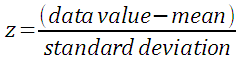
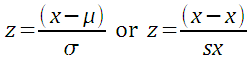
Note the parentheses!
Data that is two standard deviations below the mean will have a z-score of −2, data that is two standard deviations above the mean will have a z-score of +2. Data beyond two standard deviations away from the mean will have z-scores below −2 or above 2.

Suppose a test has a mean score of 10 and a standard deviation of 2 with a total possible of 20. Suppose a second test has the same mean of 10 and total possible of 20 but a standard deviation of 8.
On the first test a score of 18 would be rare, an unusual score. On the first test 89% of the students would have scored between 6 and 16 (three standard deviations below the mean and three standard deviations above the mean.
On the second test a score of 18 would only be one standard deviation above the mean. This would not be unusual, the second test had more spread.
Adding two scores of 18 and saying the student had a score of 36 out of 40 devalues what is a phenomenal performance on the first test.
Converting to z-scores, the relative strength of the performance on test one is valued more strongly. The z-score on test one would be (18-10)/2 = 4, while on test two the z-score would be (18-10)/8 = 1. The unusually outstanding performance on test one is now reflected in the sum of the z-scores where the first test contributes a sum of 4 and the second test contributes a sum of 1.
When values are converted to z-scores, the mean of the z-scores is zero. A student who scored a 10 on either of the tests above would have a z-score of 0. In the world of z-scores, a zero is average!
Z-scores also adjust for different means due to differing total possible points on different tests.
Consider again the first test that had a mean score of 10 and a standard deviation of 2 with a total possible of 20. Now consider a third test with a mean of 100 and standard deviation of 40 with a total possible of 200. On this third test a score of 140 would be high, but not unusually high.
Adding the scores and saying the student had a score of 158 out of 220 again devalues what is a phenomenal performance on test one. The score on test one is dwarfed by the total possible on test three. Put another way, the 18 points of test one are contributing only 11% of the 158 score. The other 89% is the test three score. We are giving an eight-fold greater weight to test three. The z-scores of 4 and 1 would add to five. This gives equal weight to each test and the resulting sum of the z-scores reflects the strong performance on test one with an equal weight to the ordinary performance on test three.
Z-scores only provide the relative standing. If a test is given again and all students who take the test do better the second time, then the mean rises and like a tide "lifts all the boats equally." Thus an individual student might do better, but because the mean rose, their z-score could remain the same. This is also the downside to using z-scores to compare performances between tests - changes in "sea level" are obscured. One would have to know the mean and standard deviation and whether they changed to properly interpret a z-score.