MS 150 Statistics Spring 2006 Mx • Name:
The data in this midterm is adapted from tables contained in the Documentation of the Traditional Food System of Pohnpei (DOTFSP), a project of the
Island Food Community of Pohnpei and the
Centre for Indigenous People's Nutrition and Environment. Due to the particular needs of a statistics examination, the data has been adapted for the examination. The data, while based in actual data from a single village on Pohnpei, should be considered in the same vein as those "based on actual events" made-for-television movies. Please refer to the
Island Food Community of Pohnpei web site for substantive and accurate information! My thanks to the Island Food Community of Pohnpei for helping provide data relevant to our students here at the college.
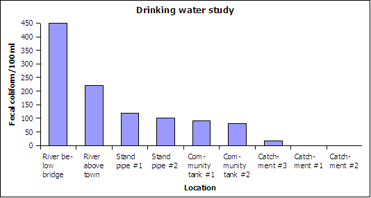
Part I: Chart
Drinking water study on fecal contamination July 2005

- _______________ What type of chart is depicted above?
Blood sugar
| mg/dl |
|---|
| 86 |
| 89 |
| 94 |
| 100 |
| 100 |
| 106 |
| 110 |
| 131 |
| 158 |
| 196 |
Part II: Basic statistics, frequencies, histogram, and z-scores.
The following section is based on data from page 49 of the DOTFSP. The data used the mean fasting blood sugar in mg/dl for females age 20 to 29 years old. The ten data points in the table on the right represent ten fictitious females. Although the sample is fictitious, the minimum, maximum, range, mean, and standard deviation match that found in the DOTFSP for this age cohort.
- __________ What level of measurement is the blood sugar data?
- __________ Find the sample size n for the blood sugar data.
- __________ Find the minimum blood sugar.
- __________ Find the maximum blood sugar.
- __________ Find the range of the blood sugar.
- __________ Find the median blood sugar.
- __________ Find the mode for the blood sugar.
- __________ Find the sample mean x blood sugar.
- __________ Find the sample standard deviation sx for the blood sugar.
- __________ Find the sample coefficient of variation CV.
- __________ If this data were to be divided into five bins, what would be the width of a single bin?
- Determine the frequency and calculate the relative frequency using five bins. Record your results in the table provided.
Frequency table
| Bins (x) | Frequency (f) | Rel. Freq. p(x) |
|---|
| _______ | _______ | _______ |
| _______ | _______ | _______ |
| _______ | _______ | _______ |
| _______ | _______ | _______ |
| _______ | _______ | _______ |
| Sum: |
_______ | _______ |
- Sketch a relative frequency histogram chart of the data here or on the back, labeling your horizontal axis and vertical axis as appropriate.
- ____________________ What is the shape of the distribution?
- ____________________ The men aged 15 to 19 have a mean blood sugar µ of 105 with standard deviation σ of 13. One young man has a blood sugar of 108. Is this an ordinary or unusual value based on the z-score?
- ____________________ The females aged 15 to 19 have a mean blood sugar µ of 94 with standard deviation σ of 15. One young woman has a blood sugar of 130. Is this an ordinary or unusual value based on the z-score?
Part III: Calculation of Mean from Frequency Table
The mean body mass was determined for 167 men and women of all ages. Use the following table to estimate the population mean body mass. [Note: this data was artificially derived from mean blood sugar cohort data binned by age on page 49 and thus the result does not represent the true population mean.]
Body Mass Index distribution (data has been rounded)
| BMI bin (x) | Freq | RF or p(x) | x*p(x) |
|---|
| 27 | 11 | 0.07 | 1.8 |
| 29 | 62 | 0.37 | 10.8 |
| 31 | 49 | 0.29 | 9.1 |
| 33 | 20 | 0.12 | 4.0 |
| 35 | 25 | 0.15 | 5.2 |
| Sums: | 167 | 1.00 | 30.9 |
|---|
- __________ What is the mean body mass index (BMI)?
- __________ A BMI between 25 and 29 is overweight, a BMI greater than or equal to 30 is obese. Does the mean body mass index indicate that, on average, the population is overweight, obese, or neither?
Part IV: Linear regression
The following data uses the mean Body Mass Index (mean BMI) data for 85 women. The first column is the mid-interval age in years for a cohort of women. The second column is the mean body mass index for that age group. This data derives from page 47 of the DOTFSP.
BMI by age
| Age cohort (x) | mean BMI (y) |
|---|
| 17 | 28.5 |
| 27 | 30.5 |
| 37 | 33.1 |
| 47 | 33.8 |
| 57 | 31.3 |
| 67 | 35.9 |
- __________ Calculate the slope of the linear trend line for the data.
- __________ Calculate the y-intercept for the data.
- __________ Is the correlation positive, negative, or neutral?
- __________ Determine the correlation coefficient r.
- __________ Is the correlation none, low, moderate, high, or perfect?
- __________ Does the relationship appear to be linear or non-linear?
- __________ Determine the coefficient of determination.
- __________ What percent in the variation in age accounts for the variation in the BMI?
- __________ What is the predicted mean BMI for a 32 year old female cohort?
- __________ What is the age at which the age cohort would be predicted to be equal to a mean BMI of 30, the threshold for obesity?
- __________ Is there an age group for which the mean BMI is neither overweight nor obese?
- __________ Can we predict the mean BMI for a cohort of seven year old females?
Why or why not?
Although this midterm utilizes data from one particular village on Pohnpei, other data from other villages on Pohnpei suggest that the overall health situation is probably not significantly different.
Table of statistical functions used by Excel
| Statistic or Parameter |
Symbol |
Equations |
Excel |
| Square root |
|
|
=SQRT(number) |
| Sample mean |
x |
Σx/n |
=AVERAGE(data) |
| Sample standard deviation |
sx |
|
=STDEV(data) |
| Sample Coefficient of Variation |
CV |
sx/x |
=STDEV(data)/AVERAGE(data) |
| Calculate a z value from an x |
z |
=
 |
=STANDARDIZE(x, µ, σ) |
| Slope |
b |
|
=SLOPE(y data, x data) |
| Intercept |
a |
|
=INTERCEPT(y data, x data) |
| Correlation |
r |
|
=CORREL(y data, x data) |
| Coefficient of Determination |
r² |
|
=(CORREL(y data, x data))^2 |
Statistics •
Lee Ling •
COM-FSM

