MS 150 Statistics Summer 2001 FX

Part I

Use this female adult literacy data to answer the following questions in part I. The female adult literacy rate is the percentage of adult women who can read.

1. Determine the sample size n.
   
   
2. Calculate the sample mean .
   
   
3. Determine the median.
   
   
4. Determine the mode.
   
   
5. Calculate the range.
   
   
6. Calculate the sample standard deviation sx.
   
   
7. Calculate the Coefficient of Variation.
   
   
8. Using the intervals specified in the bins column, fill in the frequency and relative frequency columns of the following table. The number in the bins column is the class upper limit.  Include the class upper limit in each interval. Include any data below 70 in the first interval.
   
   

   Bins	Frequency	Relative Frequency f/n
   70	_________	_________
   75	_________	_________
   80	_________	_________
   85	_________	_________
   90	_________	_________
   95	_________	_________
   100	_________	_________
   Sums:	_________	_________

   
   

9. Draw a histogram of the Relative Frequency data using the following chart:
   
10. What, if any, is the shape of the distribution?
    
    
11. What is the probability that the female adult literacy rate will be greater than 85 but less than or equal to 90?
    
    
12. Construct a 95% confidence interval for the population mean m female adult literacy rate using the above data.  Presume for this example that the data distribution is sufficiently normal.  Note that n is less than 30. Use the sample mean (question #2 above), sample standard deviation sx (question #6 above), and t_c to generate your error tolerance E (maximal error of estimate). 
    
    
    
    
    
    
    
    1. Degrees of freedom = __________
       
       
    2. Error tolerance E (maximal error of estimate) = _______________
       
       
    3. The 95% confidence interval for m is  ____________ < m < ____________
       
       
13.  In the following exercise use your sample mean and sample standard deviation as population parameters.  That is, use your the sample mean calculations in question #2 above for the population mean m.  Use your the sample standard deviation sx calculations in question #6 above for the population standard deviation s.  
    
    Let the null hypothesis H₀ be that the average female adult literacy rate is m as calculated by you in question number two above.  Suppose in the year 2000 the actual average female adult literacy rate for these same countries is = 93.  At an alpha a of 0.05, is this increase in the female literacy rate statistically significantly more than the present rate?
    
    Note that n is less than 30.  
    
    
    1. m = _____________ (from question #2 above)
       
       
    2. = 93
       
       
    3. sx = ____________ (from question #6 above)
       
       
    4. n = ____________
       
       
    5. What is H₀?
       
       
    6. What is H₁?
       
       
    7. What is a?
       
       
    8. Is this a one-tail or two tail test?
       
       
    9. How many degrees of freedom?
       
       
    10. Calculate the t-statistic.
        
        
    11. Calculate t-critical t_c.
        
        
    12. Make a sketch of the student's t-distribution curve including the critical value for t, the critical area, and the t-statistic.  Use the back if necessary to making a clean, clear, concise, legible, and accurate sketch.
        
        
        
    13. Do we reject H₀ or do we fail to reject H₀?
        
        
    14. Is the change in the female literacy rate significant?
        
        
        

Part II

For this part use the following data.  The adult female literacy rate is the percentage of women that country who can read.  The infant mortality rate is the number of babies per one thousand live births who die before they reach one year in age.  So, for example, in the FSM 88% of the adult women in the country can read and of 1000 babies born in the FSM in the year 2000, 33 will die before they reach their first birthday (the infant mortality estimates are for the year 2000). Note that the table continues across the page break.

1. Determine the slope of the least squares line (best fit) for the adult female literacy rate and infant mortality data above.
   
   
   
2. What does of the sign of the slope tell us about this data?  That is, what type of correlation is this, positive or negative?
   
   
3. Determine the y-intercept of the least squares line for the adult female literacy rate and infant mortality data above.
   
   
4. Write the equation of the least squares line for the adult female literacy rate and infant mortality data above.
   
   
   
5. Calculate the linear correlation coefficient r for the adult female literacy and infant mortality columns.
   
   
6. Is the correlation none, low, moderate, high, or perfect?
   
   
7. Calculate the coefficient of determination.
   
   
8. What does the coefficient of determination tell us about the relationship between adult female literacy rate and infant mortality rates?
   
   
   
   
9. Is there a relationship between adult female literacy (the ability of women to read) and infant mortality?
   
   
   
10. Explain what policies or programs a country might want to promote to reduce infant mortality rates based on our data.  Use the back as necessary.
    
    

Statistic or Parameter	Symbol	Equations	Excel
Square root			=SQRT(number)
Sample size	n		=COUNT(data)
Minimum			=MIN(data)
Maximum			=MAX(data)
Median			=MEDIAN(data)
Mode			=MODE(data)
Sample mean		Sx/n	=AVERAGE(data)
Population mean	m	SX/N x P(x) n p (binomial)	=AVERAGE(data)
Sample standard deviation	sx		=STDEV(data)
Population standard deviation	s	(binomial)	=STDEVP(data)
Sample variance	(sx)²		=VAR(data)
Population variance	s²		=VARP(data)
Sample Coefficient of Variation	CV	100(sx/)	=100*STDEV(data)/AVERAGE(data)
Slope	b		=SLOPE(y data, x data)
Intercept	a		=INTERCEPT(y data, x data)
Correlation	r		=CORREL(y data, x data)
Coefficient of Determination	r²		=(CORREL(y data, x data))^2
Binomial probability		nCr pr q(n-r)	=COMBIN(n,r)*p^r*q^(n-r)
Calculate a z value from an x	z	=	=STANDARDIZE(x, m, s)
Calculate an x value from a z	x	= s z + m	= s*z+m
Calculate a z-statistic from an value given m and s	z		=STANDARDIZE(, m, s/SQRT(n))
Calculate a t-statistic or t-ratio or tdata	t		=STANDARDIZE(, m, sx/SQRT(n))
Find a probability p from a z value			=NORMSDIST(z)
Find a z value from a probability p			=NORMSINV(p)
Standard error of the population mean	SE
Standard error of the sample mean	SE
Determining z critical from a for confidence intervals.	zc		=NORMSINV(1-a/2)
Error tolerance E of a mean for n ³ 30 using s	E		=CONFIDENCE(a,s,n)
Error tolerance E of a mean for n ³ 30 using sx	E		=CONFIDENCE(a,sx,n)
Error tolerance E of a mean for n < 30.  Can also be used for n ³ 30.	E		[no Excel function, determine tc and then multiply by standard error of the mean as shown in the equation]
Determining tc from a and the degrees of freedom df for a confidence interval.	tc		=TINV(a,df)
Calculate an value from a tc, sx, n, and m		=+ m
Calculate a confidence interval for a population mean m from a sample mean and an error tolerance E		-E< m <+E

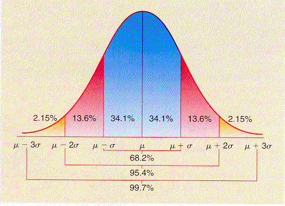
Standard normal distribution information:

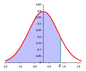
The standard normal Excel functions such as NORMSDIST and NORMSINV use "left" to z as shown at the right below:

Sources:

http://www.odci.gov/cia/publications/factbook/fields/infant_mortality_rate.html
http://www.overpopulation.com/267
http://www.cia.gov/cia/publications/factbook/indexgeo.html
http://www.adb.org/Statistics/Poverty/TUV.asp
http://www.mrdowling.com/800growth.html
http://www.unescap.org/stat/statdata/kiribati.htm
http://www.immigration-usa.com/wfb/wallis_and_futuna_people.html
http://www.overpopulation.com/1507
http://www.library.uu.nl/wesp/populstat/Oceania/naurug.htm
http://www.unicef.org/statis/Country_1Page179.html
http://www.unctad.org/en/docs/ldc99stat_tuv.en.pdf
http://www.abc.net.au/ra/pacific/places/infant_mortality.htm
http://www.adb.org/Statistics/Poverty/KIR.asp

Statistic home Lee Ling home COM-FSM home page