An item analysis of the final examination was performed with student success rates measured for each item on the final examination. The final examination is based closely on the outcomes specified on the outline.
The following table lists the concept covered on the final examination, student performance as the percent getting that question correct on the fall 2007 final examination (n = 42), a z-score calculation, and the corresponding specific student learning outcome found on the outline. The course level student learning outcomes are also listed for reference. Note that some specific student learning outcomes on the outline are not tested on the final, these are tested by other instruments during the course of the term. There are also items on the present day final that do not directly correspond to an existing student learning outcome. These will be addressed further below.
| ref | Final exam question concept/topic | fx 2007 | z | Specific learning outcomes on outline (cSLOs in bold on blue) |
| 1 | Calculate basic statistics | |||
| 2 | Distinguish between a population and a sample (define) | |||
| 3 | Distinguish between a statistic and a parameter (define) | |||
| 4 | Identify different levels of measurement when presented with nominal, ordinal, interval, and ratio data. (define) | |||
| 5 | sample size | 93% | 0.92 | Determine a sample size (calculate) |
| 6 | min | 100% | 1.29 | Determine a sample minimum (calculate) |
| 7 | max | 100% | 1.29 | Determine a sample maximum (calculate) |
| 8 | range | 93% | 0.92 | Calculate a sample range (calculate) |
| 9 | midrange | 38% | -1.89 | |
| 10 | mode | 95% | 1.05 | Determine a sample mode (calculate) |
| 11 | median | 98% | 1.17 | Determine a sample median (calculate) |
| 12 | mean | 95% | 1.05 | Calculate a sample mean (calculate) |
| 13 | standard dev | 95% | 1.05 | Calculate a sample standard deviation (calculate) |
| 14 | coef var | 93% | 0.92 | Calculate a sample coefficient of variation (calculate) |
| 15 | Represent data sets using histograms | |||
| 16 | bin width | 76% | 0.07 | Calculate a class width given a number of desired classes (calculate) |
| 17 | frequency table | 55% | -1.03 | Determine class upper limits based on the sample minimum and class width (calculate) |
| 18 | Calculate the frequencies (calculate) | |||
| 19 | Calculate the relative frequencies (probabilities) (calculate) | |||
| 20 | histogram chart | 29% | -2.38 | Create a frequency histogram based on calculated class widths and frequencies (represent) |
| 21 | Create a relative frequency histogram based on calculated class widths and frequencies (represent) | |||
| 22 | shape of distribution | 79% | 0.19 | Identify the shape of a distribution as being symmetrical, uniform, bimodal, skewed right, skewed left, or normally symmetric. (define) |
| 23 | z-score | 76% | 0.07 | |
| 24 | z ordinary/extraordinary | 74% | -0.05 | |
| 25 | z-score | 74% | -0.05 | |
| 26 | z ordinary/extraordinary | 81% | 0.31 | |
| 27 | inference from statistics | 74% | -0.05 | |
| 28 | Estimate a mean from class upper limits and relative frequencies using the formula Sx*P(x) here the probability P(x) is the relative frequency. (estimate) | |||
| 29 | Solve problems using normal curve and t-statistic distributions including confidence intervals for means and hypothesis testing | |||
| 30 | Discover the normal curve through a course-wide effort involving tossing seven pennies and generating a histogram from the in-class experiment. (develop) | |||
| 31 | Identify by characteristics normal curves from a set of normal and non-normal graphs of lines. (define) | |||
| 32 | Determine a point estimate for the population mean based on the sample mean (calculate) | |||
| 33 | Calculate a z-critical value from a confidence level (calculate) | |||
| 34 | standard error | 74% | -0.05 | |
| 35 | t-critical | 81% | 0.31 | Calculate a t-critical value from a confidence level and the sample size (calculate) |
| 36 | margin of error E | 67% | -0.42 | Calculate an error tolerance from a t-critical, a sample standard deviation, and a sample size. (calculate) |
| 37 | Solve for a confidence interval based on a confidence level, the associated z-critical, a sample standard deviation, and a sample size where the sample size is equal or greater than 30. (solve) | |||
| 38 | confidence interval | 57% | -0.91 | Solve for a confidence interval based on a confidence level, the associated t-critical, a sample standard deviation, and a sample size where the sample size is less than 30. (solve) |
| 39 | inference from statistics | 67% | -0.42 | Use a confidence interval to determine if the mean of a new sample places the new data within the confidence interval or is statistically significantly different. (interpret) |
| 40 | inference from statistics | 69% | -0.30 | |
| 41 | mean | 100% | 1.29 | |
| 42 | mean | 100% | 1.29 | |
| 43 | inference from statistics | 90% | 0.80 | |
| 44 | degrees of freedom | 69% | -0.30 | |
| 45 | t-critical | 64% | -0.54 | |
| 46 | standard error two independent samples | 48% | -1.40 | |
| 47 | margin of error E | 38% | -1.89 | |
| 48 | confidence interval for a difference of means for two indepent samples | 40% | -1.77 | |
| 49 | confidence interval hyp test for two independent samples | 69% | -0.30 | |
| 50 | Determine and interpret p-values | |||
| 51 | Calculate the two-tailed p-value for a single sample against a known population mean using a sample mean, sample standard deviation, sample size, and expected population mean along with a t-statistic. (calculate) | |||
| 52 | p-value from t-test function for paired samples and two independent samples | 95% | 1.05 | |
| 53 | inference from statistics | 81% | 0.31 | |
| 54 | inference from statistics | 71% | -0.18 | Infer from a p-value the largest confidence interval for which a change is not significant. (interpret) |
| 55 | maximum level of confidence c | 67% | -0.42 | |
| 56 | Perform a linear regression and make inferences based on the results | |||
| 57 | slope | 90% | 0.80 | Calculate the slope of the least squares line. (Calculate) |
| 58 | intercept | 90% | 0.80 | Calculate the intercept of the least squares line. (Calculate) |
| 59 | positive or negative relation | 36% | -2.01 | Identify the sign of a least squares line: positive, negative, or zero. (Define) |
| 60 | correlation r | 93% | 0.92 | Calculate the correlation coefficient r. (Calculate) |
| 61 | strength of relationship | 71% | -0.18 | Use a correlation coefficient r to render a judgment as to whether a correlation is perfect, high, moderate, low, or none. (Interpret) |
| 62 | coefficient of determination | 93% | 0.92 | Calculate the coefficient of determination r². (Calculate) |
| 63 | perc var x that explains var y | 69% | -0.30 | |
| 64 | predict y given x | 60% | -0.79 | Solve for a y value given an x value and the slope and intercept of a least squares line. (Solve) |
| 65 | predict x given y | 52% | -1.16 | Solve for a x value given an y value and the slope and intercept of a least squares line. (Solve) |
| 66 | mean | 75% | ||
| 67 | stdev | 19% |
The overall average student success rate was 75%. This represents 32 of 42 students answering correctly on average. The highest success rates are 42 correct answers out of 42 papers - 100% - for calculations of the minimum value in a data set, the maximum, and two calculations of the mean.
The z-scores provide information on areas of high and low success rates. The distribution for the z values is not symmetric due to the non-continuous nature of the data. There are no rates below 0% nor above 100%, and at 75% the mean is closer to the maximum possible success rate than the lowest possible success rate. With this in mind, the areas of high success are tinted green, and the areas of low success are tinted red.
High success rates are seen for many of the basic statistical measures (reference numbers six through thirteen). Low success rates are seen on items that are the result of a sequence of multiple calculations steps - each step appears to increase the risk of an error being introduced into the chain of calculations. The low success rate seen on reference number 59 is likely due to the intercept being negative (reference number 58). Students apparently confused the negative intercept with a negative relationship.
Some of the material on the final examination that does not have a matching specific student learning outcome represents in part the evolution of the course. In 2000 I took over the course from John Gann. The design was based closely on that former chair Stephen Blair and subsequent chair John Gann. Over time I have evolved the course, putting a greater emphasis on confidence intervals and adding the use of confidence intervals to perform hypothesis tests. This evolution was not well supported by the traditionalist Brase and Brase text in use at that time. An alternate text by Triola included the more modern emphasis on confidence intervals, and added a focus on relative standing (z-scores) in the sections on basic statistics. The Triola text, however, was almost double the price of the Brase and Brase text. In addition, Triola included material not pertinent to the course. The examples in the text focused on using Microsoft Excel and a custom built statistics add-in for Excel. The laboratory uses OpenOffice.org Calc and could not use the add-in specific examples.
I wanted a text that did not use any add-ins - even the Microsoft "Analysis" add-in requires administrative access to a Windows computer and the original operating system CD, something a graduate might not have. I wanted students to be able to run statistical calculations with a "plain vanilla" installation of a spreadsheet. The text in use this past term was custom designed to provide support for both OpenOffice.org Calc and Microsoft Excel. In an assessment of the new text, the text was well received by the students. Having a custom text has permitted the course to include a stronger emphasis on confidence intervals. Another benefit is that the reading level is closer to that of the students in the course.
The material on the final examination that does not have matching specific student learning outcomes provides useful information on changes that will eventually have to be reflected on the outline. This information will be useful to my work on a revised outline. An initial submission during the fall term was rejected by the curriculum committee. At that time I opted not to resubmit the outline pending an assessment of the new text at term's end. The end of the term has also brought useful information on what can be covered during a term using the next text. Performance in one area over multiple terms
A small assessment study done in the fall of 2006 permitted a repeated study on quiz four this fall term. That data was updated to include the fall final examination.
| Fall 2005 fx | Fall 2006 fx | Fall 2007 q04 | Fall 2007 fx | sSLO |
| 95% | 29% | 94% | 90% | Calculate the slope of the least squares line. (Calculate) |
| 95% | 92% | 90% | 90% | Calculate the intercept of the least squares line. (Calculate) |
| 65% | 92% | 100% | 36% | Identify the sign of a least squares line: positive, negative, or zero. (Define) |
| 53% | 90% | 54% | 60% | Solve for a y value given an x value and the slope and intercept of a least squares line. (Solve) |
| 45% | 48% | 46% | 52% | Solve for a x value given an y value and the slope and intercept of a least squares line. (Solve) |
| 91% | 37% | 94% | 93% | Calculate the correlation coefficient r. (Calculate) |
| 82% | 92% | 94% | 71% | Use a correlation coefficient r to render a judgment as to whether a correlation is perfect, high, moderate, low, or none. (Interpret) |
| 98% | 42% | 88% | 93% | Calculate the coefficient of determination r². (Calculate) |
| 73% | 94% | 65% | 69% | Calculate amount of variation in dependent variable explained by variation in independent variable. (Calculate) |
| 76% | 63% | 100% | NA | Based on analysis, infer whether a linear regression is appropriate? (Interpret) |
| 77% | 68% | 82% | 73% | Averages |
| 18% | 27% | 20% | 15% | stdev |
| 2.2 | 2.2 | 2.2 | 2.23 | tcritical |
| 13% | 19% | 14% | 11% | E |
At the time of quiz 04 on the 21st of September the linear regression material was fresh in the minds of the students. During the December final, the material was long out of practice. The overall success rate of 73% splits the difference between the 68% performance on the fall 2006 final and the 77% performance on the fall 2005 final. The margins of error for these indicate that they are not statistically significantly separated. These performance levels are well in line with the usual average success rate on quizzes, tests, midterm, and final. This term the average for all quizzes, tests, the midterm, and final is 65%. That average includes instances of scores of zero for students who stopped attending the course but who had not yet officially withdrawn from the class - that is, the term average will be slightly lower than the actual "live population" average.
The above table spans three textbooks and was originally generated in the fall of 2006 to look at the impact of the Triola text. The apparent drop in performance was not "real" - it is not statistically significant. In retrospect, whether the effectiveness of the texts can be inferred is highly unlikely. The present text, Introduction to Statistics Using OpenOffice.org Calc, is based on notes that were and still are available to students on the course web site. This is a confounding factor that cannot be separated out. Students may have been relying on the more readable notes during previous terms.
Course level student learning outcomes performance success rate by instrument
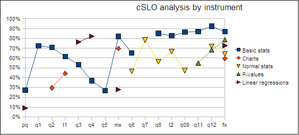
The individual item analysis data was aggregated by the five course level outcomes. Performance on aggregate in the five major areas across the term is tracked in the following chart.
Performance is over 70% on aggregate in three of the five areas. Basic statistical knowledge saw an 87% success rate on aggregate. Construction of frequency tables and associated histograms and charts was the weakest performance area. Aggregate performance on course level student learning outcomes
Aggregating the above data into a single cumulative average across the term yields the following chart.
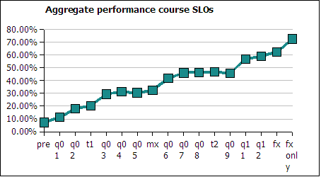
The last data point is the non-cumulative final examination performance. Due to asymmetries in the underlying number of items in each area, the final examination average as measured this way comes in at 72% instead of 75%. This is the average performance counting each course level outcome at one fifth of the weight. On the actual final examination the questions are not distributed as an even 20% in each area. There are more questions in the higher achieving basic statistics area than in lower achieving areas such as histograms and charts, the actual average on the final was 75%.
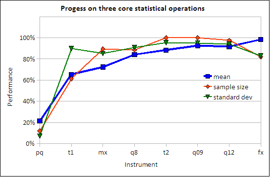
Performance on three core statistical operations
At the end of statistics course one would hope that students will be able to calculate a mean, a standard deviation, and determine the sample size. These are core concepts that appear over and over again throughout the term. Tracking these three provides an image of the learning curve and practice effect. Of interest is the fall off for two concepts on the final. There is little doubt, given the preceding track record, that almost all students had mastered these calculations. That final downturn may be evidence of the impact of final examination stresses or other external factors.
Conclusions
Areas of weakness can be specifically targeted both in the course and in future editions of the text books. One powerful strength of owning the text book is this ability to adjust the text to target the weak areas of learning. Student feedback on the text provides specific suggestions for these improvements.
Many thanks to those at the college who have supported my ongoing experimentation with my courses and who have supported the development of a text for the course.