Very Basic Excel
Today we will
learn a few basic things about Excel and then I will show you how to arrange a
grade book.
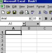
Open the Excel
program—you should find it on the desktop or in the Programs menu. You will find yourself in a blank notebook
filled with empty rectangles. The
rectangles are called cells and are where you enter data and formulas.
|
|
The
cells are referenced by column and row.
The cell in the upper left corner is cell A1. The cell next to it is cell B1. The
cell below A1 is A2, etc. |
|
|
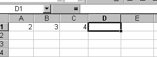
Enter
the number 2 in A1, 3 in A2 and 4 in A3.
We are now going to have Excel do some calculations on this data. |
|
|
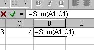
In
D1 we are going to enter a formula.
This formula will tell Excel to add up the numbers we just
entered. Formulas start with an equal
sign “=”. Click on D1 and type “=Sum(A1:C1)”.
Hit Enter. D1 will now contain
the sum of the numbers in Row 1 from Col A to Col C. |
|
|
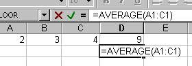
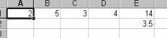
Let’s
find the average of the numbers. In
D2 type “=AVERAGE(A1:C1)” and hit Enter. You should see 3 in D2. |
|
|
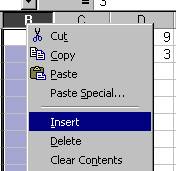
Now
we will insert a new column. Click on
the B that heads up Col B. Right
click the mouse and select Insert. A
new blank column is inserted into the spreadsheet. Now click on E1—the formula now says “SUM(A1:D1)”—it
has been updated to include the new column.
D2 is also updated. |
|
|
Enter
“5” in B1. Notice that the sum and
average are automatically updated. |
|
|
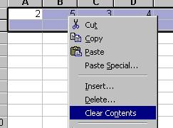
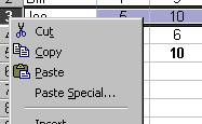
Let’s
get rid of the data we entered. Place
the pointer on A1, click down and drag to highlite all the cells in columns A
to D and rows 1 and 2. Left-click and select “Clear Contents”. (Shortcut—hit the delete key). All the data and formulas entered will be
deleted. |
|
|
|
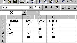
Let’s enter some data for student grades. We will enter:
Notice the Toolbar that starts with “Arial”. If you don’t see this, go to the View menu -> Toolbars -> Formatting. You
can use this toolbar for formatting.
To bold the headings, select them and click the “B”. To center data, select it and press the
button with the centered lines. |
|
|
|
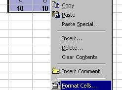
We
should make sure Excel treats our scores as numbers. Highlite the scores and totals,
right-click and select “Format Cells…” |
|
|
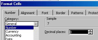
Click
the Number tab, select Number and set the Decimal places to 0. |
|
|
Kevin
just added the class. We need to add
him to the list. Click the number 3
to highlite row 3. Right click and
select Enter. A new row is entered. Click
on A3 and enter data for Kevin. |
|
|
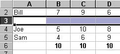
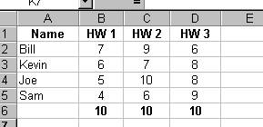
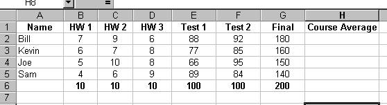
Here
is the current spreadsheet. |
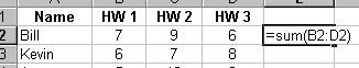
Before
finishing the grade book, let’s practice a bit with formulas. Suppose we wanted to know the total number
of homework points earned by each student.
We would use a Sum() formula.
Click on E2 and enter the formula to sum up Bill’s homework points.
|
|
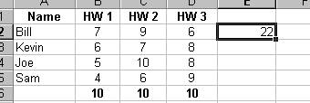
Don’t
forget to use the “=” before typing the formula. Hit
Enter and it looks like this. We
could enter a similar formula for each student, but this is tedious. We will “DRAG” the formula down. Place
the white cross on the lower right-hand corner of E2(it should turn into a
black cross), click and hold the left-button on the mouse and drag down to
E5. Then release the button. |
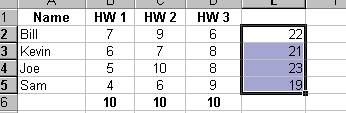
Click
on E2 and look at the formula in the formula bar. Now use the down arrow to move down through the rows. Observe that Excel updated the formula on
each row to sum the scores in that row.
Delete these formulas, as we won’t be needing them. We will finish the grade book…
Let’s
suppose we had two tests each worth 100 points and a final exam worth 200
points. Create headings and enter
scores for each of the students.
|
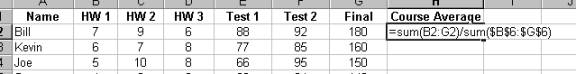
I
have created data for two tests, a final exam and added a column where the
final average for the course will be calculated. A bit of mathematics—the course average for Bill is the sum of
his scores divided by the sum of the totals in Row 6. Enter the formula like this: “=sum(B2:G2)/sum($B$6:$G$6)” |
|
|
So
what are all those dollars signs ($)
about? When we drag down the formula,
we want the cell references in the numerator of formula to be updated for each
row, but we want the references in the denominator to stay the same for each
student. The “$”
tells Excel to keep that cell reference the same for each row as the formula is
dragged down.
|
Enter
the formula like above and type enter.
Then drag down to Row 6.
Format the cells in Col H to be numbers with 2 decimal places. |
|
|
|
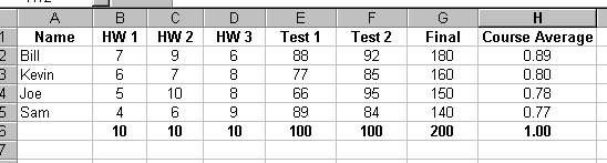
Here
is what my spreadsheet looks like. I
have centered the data and emboldened the bottom row. If you do not have the number “1.00” in
the last column of the totals row, then you have made a mistake in your
formulas. The “Course Average” is in
decimal form. For example, Bill has
an 89% average for the course. |
|
|
Here
are some exercises you can try:
1)
Suppose Kevin
complains that he deserved a better score on his first test. Update his first test score and watch how
his course average is automatically updated.
2)
Make the
Course Average be displayed as percentages.
There are several ways to do this.
One is to rewrite to formula.
Another is to use the “Format Cells” option.