
Confidence intervals for n ≥ 30 Confidence intervals for n < 30 Deciding on a sample size
In many formulas we have used the population mean µ. Two chapters ago we used the formula: z = (x - µ)/σ
In the previous chapter we used the related formula:
In these and other sections we have been given the value of µ and σ. We often do statistical studies, however, exactly because we do not know µ or σ. We do statistical studies of a sample and generate a sample mean x and a sample standard deviation sx.
If n ≥ 30 then σx is roughly equal to sx (the population standard deviation = sample standard deviation).
You might recall that the formula for the sample standard used an n-1 in the denominator. This makes the sample stdev slightly larger: better to overestimate σ than underestimate σ and risk portraying the data as more precise than it actually is.
We say that the sample standard deviation is a point estimate for the population standard deviation.
Whenever we use a single statistic to estimate a parameter we refer to the estimate as a point estimate for that parameter.
As a point estimate for the population mean µ we use the sample mean x.
The error of a point estimate is the magnitude of estimate minus the actual parameter (where the magnitude is always positive). The error in using x for µ is ( x - µ ). Note that to take a positive value we need to use either the absolute value |( x - µ )| or √( x - µ )2.
Note that the error of an estimate is the distance of the statistic from the parameter.
Unfortunately, the whole reason we were using x is because we did not know µ.
For example, given the mean body fat index (BFI) of 51 male students at the national campus is x = 19.9 with a sample standard deviation of sx = 7.7, what is the error |( x - µ )| if µ is the average BFI for male COMFSM students?
We can't calculate this. We do not know µ! So we say µ is a point estimate for x. That would make the error equal to zero and implies that our sample mean x is exactly the same as µ.
Is x really the exact value of µ for all the males at the national campus? Probably not!
We might be more accurate if we were to say that the mean µ is somewhere between two values.
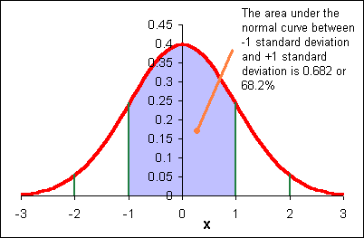
Here is a key point: remember that the sample mean x distributes normally with a standard deviation of σ/√n. We will use sx to estimate σ. That means that if I set my estimate for µ to be between x - sx/√n and x + sx/√n, then there is a 0.682 probability that µ will be included in that interval.
x - sx/√n ≤ µ ≤ x + sx/√n
19.9 - 7.7/sqrt(51) ≤ µ ≤ 19.9 + 7.7/sqrt(51)
19.9 - 1.1 ≤ µ ≤ 19.9 + 1.1
18.8 ≤ µ ≤ 21.0
Of course that also means that there is a 0.318 probability we have not included m in our interval. Think of this as a 32% chance of being wrong: a one in three chance we have not included µ in the interval. Do you want to be wrong one in three times?
So expand the interval to x - 2*sx and x - 2*sx:
x - 2*sx/√n ≤ µ ≤
x + 2*sx/√n
19.9 - 2*7.7/sqrt(51) ≤ µ ≤ 19.9 + 2*7.7/sqrt(51)
19.9 - 2.2 ≤ µ ≤ 19.9 + 2.2
17.7 ≤ µ ≤ 22.1
Now we have a 0.9545 probability that µ is within our interval. We might say we are "95.45%" certain we have encompassed µ. We call this a "95.45%" confidence interval for our population mean µ. We have a 0.0455 probability that our interval will not encompass the population mean µ.
Note the structure of the above:
x - z*sx/√>n ≤ µ ≤ x + z*sx/√n
If we say the Error E = z*sx/√n then we can write
x - E ≤ µ ≤ x + E
So the next logical step is to decide how often, as a probability, we want to be "right." If we want the probability of including the population mean µ to be 68.2%, then we use z = 1. If we want the probability that our interval includes the population mean µ to be 95.45%, then we use a z = 2. These "probabilities of being right" are termed levels of confidence, the intervals are called confidence intervals.
The confidence level often varies with the particular field of research. In engineering, physics, and medicine we usually want to be very confident that we have included the mean. Confidence intervals based on a level of confidence of 99% and 99.5% are often used. In education, athletics, and the social sciences we often use a confidence level of 95% or, depending on the situation, 90%.
Suppose we decide to use a confidence level of 95%. This means a value of z near z = 2. But z = 2 produces a confidence interval of 95.45%. What we are really asking for are the ± z values that include 95% of the area under the normal curve. Finding a z value from a probability means using the NORMSINV function in Excel.
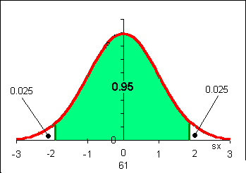
To find the z-value that includes 0.95 of the area under the normal curve we need to use =NORMSINV(0.025). Why the normal curve? Because the sample mean distribution always distributes normally for n ≥ 30. Why 0.025 and not 0.05? Use a sketch: there are "two tails" each with half the area of 0.05. To get the correct z value we can calculate the z value for the area in the left "tail" only.
zc = NORMSINV(0.025) = -1.96
This is the negative (rightmost) value for zc, the right value is simply the absolute value: 1.96. We usually write zc as the positive (or absolute) value of the number returned by the NORMSINV function.
Note the subscript c on the z: we refer to the z values associated with a confidence interval as "z-critical" values or zc.
We can calculate the 95% confidence interval the same way we calculated the 68% and the 95.45% confidence interval:
x - zc*sx/√n ≤ µ ≤
x + zc*sx/√n
x - 1.96*sx/√n ≤ µ ≤
x + 1.96*sx/√n
19.9 - 1.96*7.7/sqrt(51) ≤ µ ≤ 19.9 + 1.96*7.7/sqrt(51)
19.9 - 2.1 ≤ µ ≤ 19.9 + 2.1
17.8 ≤ µ ≤ 22.0
We are asserting that there is a 95% probability that the population mean µ body fat index for the males at the national campus of COM-FSM is between 17.8 and 22.0.
Note that the Error E = zc*sx/√n
In the above example the Error E = 2.1
The confidence interval is usually written as:
x - E ≤ µ ≤ x + E
where E = zc*sx
To calculate the zc for any confidence level c: =NORMSINV((1-c)/2)
Note that the result is the LEFT or negative z-critical value, use the positive value of z in the formula for E.
Example:
Given that n = 219 CHS students took the TOEFL examination with a sample mean score of x = 369 and a sample standard deviation sx = 50, construct a 90% confidence interval for the population mean TOEFL score for CHS.
The confidence interval will be given by:
x - E ≤ µ ≤ x + E
where E = zc*sx/√n and where zc is calculated using a confidence level of 0.90.
zc =NORMSINV((1-0.9)/2) = -1.6449
Use the absolute value of zc in the formula for E: (1.6449)(50)/sqrt(219)
E = zc*sx/√n = (1.6449)(50)/sqrt(219) = 5.56
Therefore the 90% confidence interval is:
x - E ≤ µ ≤
x + E
369 - 5.56 ≤ µ ≤ 369 + 5.56
363.4 ≤ µ ≤ 374.6
What if n < 30? There is an increased risk that our sample is not representative of the population. We need to increase the width of our confidence interval to increase the probability that we will include the population mean in our confidence interval. The smaller our sample size, the more we will have to increase the width of the confidence interval.
Thus these confidence intervals will depend in part on the sample size n.
We will no longer use the standard normal distribution to calculate z values. Now we will use a related distribution called the student's t-distribution to calculate a t value. The calculation of E will look almost the same as in the earlier section.
The confidence interval will still be:
x - E ≤ µ ≤ x + E
E, however, will be different for n < 30. E will be calculated using:
E = tc*sx/√n
tc will be calculated using the TINV function in Excel. The TINV function will need TWO inputs: the desired level of confidence and the DEGREES OF FREEDOM. The degrees of freedom, or df, is simply one less than the sample size: degrees of freedom = n-1.
tc =TINV(1-c,df)
Note especially that there is no need to divide by 2: the TINV function calculates the t-critical for the two-tailed case. The function also always returns the positive or rightmost t-critical value.
Example
For a sample size of n = 10 runs home, I have a sample mean time of 61 minutes with a sample standard deviation of 7 minutes. Construct a 95% confidence interval for my population mean run time.
n = 10
x = 61
sx = 7
degrees of freedom = 10 - 1 = 9
tc =TINV(1-0.95,10-1) = 2.2622
E = tc*sx/√n = (2.4469)(7)/√10 = 5.01
x - E ≤ µ ≤ x + E
61 - 5.01 ≤ µ ≤ 61 + 5.01
56.0 ≤ µ ≤ 66.0
I can be 95% confident that my population mean run time should be between 56 and 66 minutes.
Suppose you are designing a study and you have in mind a particular error E you do not want to exceed. You can determine the sample size n you'll need if you have prior knowledge of the standard deviation sx. How would you know the sample standard deviation in advance of the study? One way is to do a small "pre-study" to obtain an estimate of the standard deviation. These are often called "pilot studies."
If we have an estimate of the standard deviation, then we can estimate the sample size needed to obtain the desired error E.
Since E = zc*sx/√n, then n = (zc*sx/E)²
Suppose I want an error E = 1.0 at a confidence level of 0.95 in my study of male student body fat. I can use the sx from the sample of 51 students to estimate my necessary sample size:
n = (1.96*7.7/1)2 = 227.77 or 228 students. Thus I estimate that I will need 228 male students to reduce my error to ±1 in my body fat study.
Suppose we want a 99% confidence internal with a error E of half (0.5) of an inch in the projected height of a COMFSM College student. Presume we suspect sx = 3.45 from a preliminary study. How many students will we have to survey?
n = (zc*sx/E)2 = (2.58*3.45/0.5)2 = 317 students.
Note that zc was calculated using: =ABS(NORMSINV((1-0.99)/2)) where ABS returned the absolute value of the NORMSINV function.
We would have to survey 317 students. If we have σ, we use it, but in real life we usually just have an estimate of σ from sx.
•
Statistics •
Lee Ling •
COMFSM •