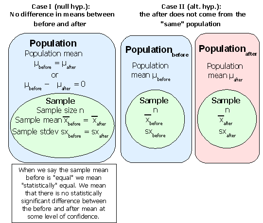
Many studies investigate systems where there are measurements taken before and after. Usually there is an experimental treatment or process between the two measurements. A typical such system would be a pre-test and a post-test. Inbetween the pre-test and the post-test would typically be an educational or training event. One could examine each student's score on the pre-test and the post-test. Even if everyone did better on the post-test, one would have to prove that the difference was statistically significant and not just a random event.
These studies are called "paired t-tests" or "inferences from matched pairs". Each element in the sample is considered as a pair of scores. The null hypothesis would be that the average difference for all the pairs is zero: there is no difference. For a confidence interval test, the confidence interval for the mean differences would include zero if there is no statistically significant difference.
If the difference for each data pair is referred to as d, then the mean difference could be written d. The hypothesis test is whether this mean difference d could come from a population with a mean difference μd equal to zero (the null hypothesis). If the mean difference d could not come from a population with a mean difference μd equal to zero, then the change is statistically significant. In the diagram above the mean difference μd is equal to μbefore − μ after.
Consider the paired data below. The first column are female body fat measurements from the beginning of a term. The second column are the body fat measurements sixteen weeks later. The third column is the difference d for each pair.
| BodyFat before | Bodyfat after | Bodyfat difference d |
|---|---|---|
| 23.5 | 20.8 | -2.7 |
| 28.9 | 27.5 | -1.4 |
| 29.2 | 28.4 | -0.8 |
| 24.7 | 24.1 | -0.6 |
| 26.4 | 26.1 | -0.3 |
| 23.7 | 24 | 0.3 |
| 46.9 | 47.2 | 0.3 |
| 23.6 | 24 | 0.4 |
| 26.4 | 27.1 | 0.7 |
| 15.9 | 17 | 1.1 |
| 30.3 | 31.5 | 1.2 |
| 28.0 | 29.3 | 1.3 |
| 36.2 | 37.6 | 1.4 |
| 31.3 | 32.8 | 1.5 |
| 31.5 | 33.2 | 1.7 |
| 26.7 | 28.6 | 1.9 |
| 26.5 | 29.0 | 2.5 |
The confidence interval is calculated on the differences d (third column above) using the sample size n, sample mean difference d, and the sample standard deviation of the difference data d. The following table includes calculations using a 95% confidence interval.
| Count of the differences | 17 |
| sample mean difference d | 0.50 |
| Standard deviation of the difference data d | 1.33 |
| Standard error for the mean of the difference data d | 0.32 |
| tc for confidence level = 0.95 | 2.12 |
| Margin of the error E for the mean | 0.68 |
| Lower bound for the 95% confidence interval | -0.18 |
| Upper bound for the 95% confidence interval | 1.18 |
The 95% confidence interval includes a possible population mean of zero. The population mean difference μd could be equal to zero.
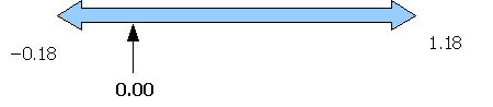
This means that "no change" is a possible population mean. To use the double negative, we cannot rule out the possibility of no change. We fail to reject the null hypothesis of no change. The women have not statistically significantly gained body fat over the sixteen weeks of the term.
Spreadsheets provide a function to calculate the p-value for paired data using the student's t-distribution. This function is the TTEST function. If the the p-value is less than your chosen risk of a type I error α then the difference is significant. The function does not require generating the difference column d as seen above, only the original data is used in this function.
The function takes as inputs the before data (data_range_x), the after data (data_range_y), the number of tails, and a final variable that specifies the type of test. A paired t-test is test type number one.
=TTEST(data_range_x,data_range_y,2,1)
To ensure that the spreadsheet calculates the p-value correctly, delete any data missing the x or y value in the pair. Data missing an x or y value is not paired data!
The maximum confidence we can have that the difference is statistically significant is 1 − p-value.
| p-value | 0.14 |
| Maximum confidence level c | 0.86 |
The p-value confirms the confidence interval analysis, we fail to reject the null hypothesis. At a 5% risk of a type I error we would fail to reject the null hypothesis. We can have a maximum confidence of only 86%, not the 95% standard typically employed. Some would argue that our concern for limited the risk of rejecting a true null hypothesis (a type I error) has led to a higher risk of failing to reject a false null hypothesis (a type II error). Some would argue that because of other known factors - the high rates of diabetes, high blood pressure, heart disease, and other non-communicable diseases - one should accept a higher risk of a type I error. The average shows an increase in body fat. Given the short time frame (a single term), some might argue for reacting to this number and intervening to reduce body fat. They would argue that given other information about this population's propensity towards obesity, 86% is "good enough" to show a developing problem. Ultimately these debates cannot be resolved by statisticians.
One of the more common situations is when one is seeking to compare two independent samples to determine if the means for each sample are statistically significantly different. In this case the samples may differ in sample size n, sample mean, and sample standard deviation.
In this text the two samples are refered to as the x data and the y data. The sample size for the x data is nx. The sample mean for the x data is x. The sample standard deviation for the x data is sx. For the y data, the sample size is ny, the sample mean is y, and the sample standard deviation is sy.
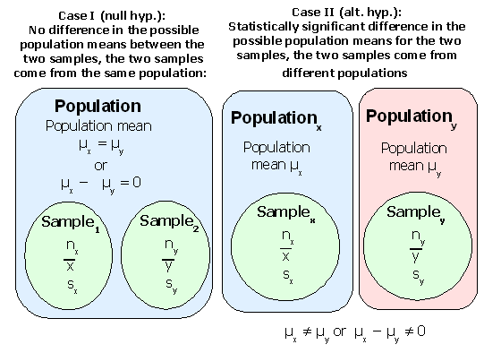
Two possibilities exist. Either the two samples come from the same population and the population mean difference is statistically zero. Or the two samples come from different populations where the population mean difference is statistically not zero.
Each sample has a range of probable values for their population mean μ. If the confidence interval for the sample mean differences includes zero, then there is no statistically significant difference in the means between the two samples. If the confidence interval does not include zero, then the difference in the means is statistically significant.
Note that the margin of error E for the mean difference is still tc multiplied by the standard error. The standard error formula changes to account for the differences in sample size and standard deviation.
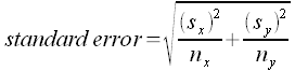
Thus the margin of error E can be calculated using:
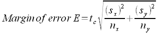
For the degrees of freedom in the t-critical tc calculation use n − 1 for the sample with the smaller size. This produces a conservative estimate of the degrees of freedom. Advanced statistical software uses another more complex formula to determine the degrees of freedom.
The confidence interval is calculated from:
(x − y) − E < (μx − μy) < (x − y) + E
Where x is the sample mean of one data set and y is the sample mean of the other data. Some texts use the symbol xd for this difference and μd for the hypothesized difference in the population means. This leads to the more familiar looking formulation:
xd − E < μd < xd + E
Where:
μd = μx − μy and
xd = x − y
Remember, μx and μy are not known. These are left as symbols. After calculating the interval, check to see if the confidence includes zero. If zero is inside the interval, then the sample means are not significantly different and we fail to reject the null hypothesis.
The following table uses a local business example. Data was recorded as to how many cup of sakau were consumed in a single night at two sakau markets on Pohnpei. The implication is that the lower the average, the stronger the sakau. The average difference, however, has to be statistically significant.
| Song mahs (x) | Rush Hour (y) | |
|---|---|---|
| 2 | 2 | |
| 3 | 10 | |
| 6 | 1.5 | |
| 3 | 5.5 | |
| 3.5 | 9 | |
| 4.5 | 7.5 | |
| 1 | 5.5 | |
| 5 | 3 | |
| 3 | 3 | |
| 7 | 6 | |
| 4 | 3 | |
| 2.5 | 4.5 | |
| 5.5 | 10 | |
| 2 | 9 | |
| 1 | 2 | |
| 2 | 2 | |
| 4 | ||
| 5 | ||
| 5 | ||
| 5.5 | ||
| 15 | ||
| 14 | ||
| 2 | ||
| 2 | ||
| 4 | ||
| Sample statistics | ||
| sample size n | 16 | 25 |
| sample mean | 3.44 | 5.6 |
| sample stdev | 1.77 | 3.73 |
| Confidence interval statistics | ||
| standard error | 0.87 | |
| t-critical tc | 2.13 | |
| margin of error E | 1.85 | |
| difference of means | -2.16 | |
| lower bound ci | -4.01 | |
| upper bound ci | -0.31 | |
Note that 15 was used for the degrees of freedom in the t-critical calculation. Sixteen is the sample size of the smaller sample.
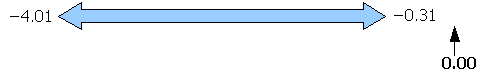
Note that the confidence interval does not include zero. The confidence interval indicates that whatever the population mean difference μd might be, the population mean μd cannot be zero. This means that the sample means are statistically significantly different. We would reject a null hypothesis of no difference between the two markets. The implication is that Song Mahs is stronger than Rush Hour, at least on these two nights.
As noted above, spreadsheets provide a function to calculate p-values. If the the p-value is less than your chosen risk of a type I error α then the difference is significant.
The function takes as inputs one the data for one if the two samples (data_range_x), the data for the other sample (data_range_y), the number of tails, and a final variable that specifies the type of test. A t-test for means from independent samples is test type number three.
=TTEST(data_range_1,data_range_2,number of tails,3)
For the above data, the p-value is given in the following table:
| p-value | 0.02 |
| Maximum confidence level c | 0.98 |
The TTEST function does not use the smaller sample size to determine the degrees of freedom. The TTEST function uses a different formula that calculates a larger number of degrees of freedom, which has the effect of reducing the p-value. Thus the confidence interval result could produce a failure to reject the null hypothesis while the TTEST could produce a rejection of the null hypothesis. This only occurs when the p-value is close to your chosen α.
[Optional material!] If you have doubts and want to explore further, take the difference of the means and divide by the standard error to obtain the t-statistic t. Then use the TDIST function to determine the p-value, using the smaller sample size − 1 to calculate the degrees of freedom.
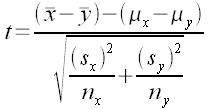
Note that (μx − μy) is presumed to be equal to zero. Thus the formula is the difference of the means divided by the standard error (given further above).
t = xd ÷ (standard error)
Once t is calculated, use the TDIST function to determine the p-value.
=TDIST(ABS(t),n−1,2)
Technical side-note: TTEST type three does not presume that the population standard deviations σx and σy are equal. This is in keeping with modern practice and reality. TTEST type two presumes σx = σy. One rarely knows either value, and if one did know those values, why would not they also know the actual population means? With the true population means in hand, then any difference would be significant.