
In this chapter we explore whether a sample has a sample mean x that could have come from a population with a known population mean μ. There are two possibilities. In Case I below, the sample mean x comes from the population with a known mean μ. In Case II, on the right, the sample mean x does not come from the population with a known mean μ. For our purposes the population mean μ could be a pre-existing mean, an expected mean, or a mean against which we intend to run the hypothesis test. In the next chapter we will consider how to handle comparing two samples to each other to see if they come from the same population.
Suppose we want to do a study of whether the female students at the national campus gain body fat with age during their years at COM-FSM. Suppose we already know that the population mean body fat percentage for the new freshmen females 18 and 19 years old is μ = 25.4.
We measure a sample size n = 12 female students at the national campus who are 21 years old and older and determine that their sample mean body fat percentage is x = 30.5 percent with a sample standard deviation of sx = 8.7.
Can we conclude that the female students at the national campus gain body fat as they age during their years at the College?
Not necessarily. Samples taken from a population with a population mean of μ = 25.4 will not necessarily have a sample mean of 25.4. If we take many different samples from the population, the sample means will distribute normally about the population mean, but each individual mean is likely to be different than the population mean.
In other words, we have to consider what the likelihood of drawing a sample that is 30.5 - 25.4 = 5.1 units away from the population mean for a sample size of 12. If we knew more about the population distribution we would be able to determine the likelihood of a 12 element sample being drawn from the population with a sample mean 5.1 units away from the actual population mean..
In this case we know more about our sample and the distribution of the sample mean. The distribution of the sample mean follows the student's t-distribution. So we shift from centering the distribution on the population mean and center the distribution on the sample mean. Then we determine whether the confidence interval includes the population mean or not. We construct a confidence interval for the range of the population mean for the sample.
If this confidence interval includes the known population mean for the 18 to 19 years olds, then we cannot rule out the possibility that our 12 student sample is from that same population. In this instance we cannot conclude that the women gain body fat.
If the confidence interval does NOT include the known population mean for the 18 to 19 year old students then we can say that the older students come from a different population: a population with a higher population mean body fat. In this instance we can conclude that the older women have a different and probably higher body fat level.
One of the decisions we obviously have to make is the level of confidence we will use in the problem. Here we enter a contentious area. The level of confidence we choose, our level of bravery or temerity, will determine whether or not we conclude that the older females have a different body fat content. For a detailed if somewhat advanced discussion of this issue see The Fallacy of the Null-Hypothesis Significance Test by William Rozeboom.
In education and the social sciences there is a tradition of using a 95% confidence interval. In some fields three different confidence intervals are reported, typically a 90%, 95%, and 99% confidence interval. Why not use a 100% confidence interval? The normal and t-distributions are asymptotic to the x-axis. A 100% confidence interval would run to plus and minus infinity. We can never be 100% confident.
In the above example a 95% confidence interval would be calculated in the following way:
n = 12
x = 30.53
sx = 8.67
c = 0.95
degrees of freedom = 12 -1 = 11
tc = tinv((1-0.95,11) = 2.20
E = tc*sx/sqrt(12) = 5.51
x - E < μ <
x + E
25.02 < μ < 36.04
The 95% confidence interval for our n = 12 sample includes the population mean 25.3. We CANNOT conclude at the 95% confidence level that this sample DID NOT come from a population with a population mean μ of 25.3.
Another way of thinking of this is to say that 30.5 is not sufficiently separated from 25.8 for the difference to be statistically significant at a confidence level of 95% in the above example.
In common language, the women are not gaining body fat.
The above process is reduced to a formulaic structure in hypothesis testing. Hypothesis testing is the process of determining whether a confidence interval includes a previously known population mean value. If the population mean value is included, then we do not have a statistically significant result. If the mean is not encompassed by the confidence interval, then we have a statistically significant result to report.
Homework
If I expand my study of female students 21+ to n = 24 and find a sample mean x = 28.7 and an sx=7, is the new sample mean statistically significantly different from a population mean μ of 25.4 at a confidence level of c = 0.90?
The null hypothesis is the supposition that there is no change in a value from some pre-existing, historical, or expected value. The null hypothesis literally supposes that the change is null, non-existent, that there is no change.
In the previous example the null hypothesis would have been H0: μ = 25.4
The alternate hypothesis is the supposition that there is a change in the value from some pre-existing, historical, or expected value. Note that the alternate hypothesis does NOT say the "new" value is the correct value, just that whatever the mean μ might be, it is not that given by the null hypothesis.
H1: μ ≠ 25.4
We run hypothesis test to determine if new data confirms or rejects the null hypothesis.
If the new data falls within the confidence interval, then the new data does not contradict the null hypothesis. In this instance we say that "we fail to reject the null hypothesis." Note that we do not actually affirm the null hypothesis. This is really little more than semantic shenanigans that statisticians use to protect their derriers. Although we run around saying we failed to reject the null hypothesis, in practice it means we left the null hypothesis standing: we de facto accepted the null hypothesis.
If the new data falls outside the confidence interval, then the new data would cause us to reject the null hypothesis. In this instance we say "we reject the null hypothesis." Note that we never say that we accept the alternate hypothesis. Accepting the alternate hypothesis would be asserting that the population mean is the sample mean value. The test does not prove this, it only shows that the sample could not have the population mean given in the null hypothesis.
For two-tailed tests, the results are identical to a confidence interval test. Note that confidence interval never asserts the exact population mean, only the range of possible means. Hypothesis testing theory is built on confidence interval theory. The confidence interval does not prove a particular value for the population mean , so neither can hypothesis testing.
In our example above we failed to reject the null hypothesis H0 that the population mean for the older students was 25.4, the same population mean as the younger students.
In the example above a 95% confidence interval was used. At this point in your statistical development and this course you can think of this as a 5% chance we have reached the wrong conclusion.
Imagine that the 18 to 19 year old students had a body fat percentage of 24 in the previous example. We would have rejected the null hypothesis and said that the older students have a different and probably larger body fat percentage.
There is, however, a small probability (less than 5%) that a 12 element sample with a mean of 30.5 and a standard deviation of 8.7 could come from a population with a population mean of 24. This risk of rejecting the null hypothesis when we should not reject it is called alpha α. Alpha is 1-confidence level, or α = 1-c. In hypothesis testing we use α instead of the confidence level c.
| Suppose | And we accept H0 as true | Reject H0 as false |
|---|---|---|
| H0 is true | Correct decision. Probability: 1 − α | Type I error. Probability: α |
| H0 is false | Type II error. Probability: β | Correct decision. Probability: 1 − β |
Hypothesis testing seeks to control alpha α. We cannot determine β (beta) with the statistical tools you learn in this course.
Alpha α is called the level of significance. 1 − β is called the "power" of the test.
The regions beyond the confidence interval are called the "tails" or critical regions of the test. In the above example there are two tails each with an area of 0.025. Alpha α = 0.05
For hypothesis testing it is simply safest to always use the t-distribution. In the example further below we will run a two-tail test.

Example
Using the data from the first section of these notes:
=
(30.53-25.4)/(8.67/sqrt(8.67)) = 2.05
Note the changes in the above sketch from the confidence interval work. Now the distribution is centered on μ with the distribution curve described by a t-distribution with eleven degrees of freedom. In our confidence interval work we centered our t-distribution on the sample mean. The result is, however, the same due to the symmetry of the problems and the curve. If our distribution were not symmetric we could not perform this sleight of hand.
The hypothesis test process reduces decision making to the question, "Is the t-statistic t greater than the t-critical value tc? If t > tc, then we reject the null hypothesis. If t < tc, then we fail to reject the null hypothesis. Note that t and tc are irrational numbers and thus unlikely to ever be exactly equal.
I have a previously known population mean μ running pace of 6'09" (6.15). In 2001 I've been too busy to run regularly. On my five most recent runs I've averaged a 6'23" (6.38) pace with a standard deviation 1'00" At an alpha α = 0.05, am I really running differently this year?
H0: μ = 6.15
H1: μ ≠ 6.15
Pay close attention to the above! We DO NOT write H1: μ = 6.23. This is a common beginning mistake.
=
(6.38-6.15)/(1.00/sqrt(5)) = 0.51
Note that in my sketch I am centering my distribution on the population mean and looking at the distribution of sample means for sample sizes of 5 based on that population mean. Then I look at where my actual sample mean falls with respect to that distribution.
Note that my t-statistic t does not fall "beyond" the critical values. I do not have enough separation from my population mean: I cannot reject H0. So I fail to reject H0. I am not performing differently than last year. The implication is that I am not slower.
Return to our first example in these notes where the body fat percentage of 12 female
students 21 years old and older was ![]() =30.53
with a standard deviation sx=8.67 was tested against a null hypothesis H0 that
the population mean body fat for 18 to 19 year old students was μ = 25.4. We failed to
reject the null hypothesis at an alpha of 0.05. What if we are willing to take a larger
risk? What if we are willing to risk a type I error rate of 10%? This would be an alpha of
0.10.
=30.53
with a standard deviation sx=8.67 was tested against a null hypothesis H0 that
the population mean body fat for 18 to 19 year old students was μ = 25.4. We failed to
reject the null hypothesis at an alpha of 0.05. What if we are willing to take a larger
risk? What if we are willing to risk a type I error rate of 10%? This would be an alpha of
0.10.
=
(30.53-25.4)/(8.67/sqrt(12)) = 2.05
With an alpha of 0.10 (a confidence interval of 0.90) our results are statistically significant. These same results were NOT statistically significant at an alpha α of 0.05. So which is correct:
Note how we would have said this in confidence interval language:
The answer is that it depends on how much risk you are willing take, a 5% chance of committing a Type I error (rejecting a null hypothesis that is true) or a larger 10% chance of committing a Type I error. The result depends on your own personal level of aversity to risk. That's a heck of a mathematical mess: the answer depends on your personal willingness to take a particular risk.
Consider what happens if someone decides they only want to be wrong 1 in 15 times: that corresponds to an alpha of α = 0.067. They cannot use either of the above examples to decide whether to reject the null hypothesis. We need a system to indicate the boundary at which alpha changes from failure to reject the null hypothesis to rejection of the null hypothesis.
Consider what it would mean if t-critical were equal to the t-statistic. The alpha at which t-critical equals the t-statistic would be that boundary value for alpha α. We will call that boundary value the p-value.
The p-value is the alpha for which tinv(α;df)=
 .
But how to solve for α?
.
But how to solve for α?
The solution is to calculate the area in the tails under the t-distribution using the tdist function. The p-value is calculated using the OpenOffice Calc formula:
=TDIST(ABS(t);degrees of freedom;number of tails)
The degrees of freedom are n − 1 for comparison of a sample mean to a known or pre-existing population mean μ.
Note that TDIST can only handle positive values for the t-statistic, hence the absolute value function.
p-value = TDIST(ABS(2.05;11;2) = 0.06501
The p-value represents the SMALLEST alpha α for which the test is statistically significant.
The p-value is the SMALLEST alpha α for which we reject the null hypothesis.
Thus for all alpha greater than 0.065 we reject the null hypothesis. The "one in fifteen" person would reject the null hypothesis (0.0667 > 0.065). The alpha = 0.05 person would not reject the null hypothesis.
If the pre-chosen alpha is more than the p-value, then we reject the null hypothesis. If the pre-chosen alpha is less than the p-value, then we fail to reject the null hypothesis.
The p-value lets each person decide on their own level of risk and removes the arbitrariness of personal risk choices.
Because many studies in education and the social sciences are done at an alpha of 0.05, a p-value at or below 0.05 is used to reject the null hypothesis.
1 − p-value is the confidence interval for which the new value does not include the pre-existing population mean. Another way to say this is that 1 − p-value is the maximum confidence level c we can have that the difference (change) is significant. We usually look for a maximum confidence level c of 0.95 (95%) or higher.
Note:
p-value = TDIST(ABS(t),n−1,number_tails)
All of the work above in confidence intervals and hypothesis testing has been with two-tailed confidence intervals and two-tailed hypothesis tests. There are statisticians who feel one should never leave the realm of two-tailed intervals and tests.
Unfortunately, the practice by scientists, business, educators and many of the fields in social science, is to use one-tailed tests when one is fairly certain that the sample has changed in a particular direction. The effect of moving to a one tailed test is to increase one's risk of committing a Type I error.
One tailed tests, however, are popular with researchers because they increase the probability of rejecting the null hypothesis (which is what most researchers are hoping to do).
The complication is that starting with a one-tailed test presumes a change, as in ANY change in ANY direction has occurred. The proper way to use a one-tailed test is to first do a two-tailed test for change in any direction. If change has occurred, then one can do a one-tailed test in the direction of the change.
Returning to the earlier example of whether I am running slower, suppose I decide I want to test to see if I am not just performing differently (≠), but am actually slower (<). I can do a one tail test at the 95% confidence level. Here alpha will again be 0.05. In order to put all of the area into one tail I will have to use the OpenOffice Calc function TINV(2*α,df).
H0: μ = 6.15
H1: μ < 6.15
μ=6.15
x = 6.38
sx = 1.00
n = 5
degrees of freedom (df)=4
tc = TINV(2*α,df) = TINV(2*0.05,4) = 2.13
t-statistic = =
(6.38-6.15)/(1.00/sqrt(5)) = 0.51
Note that the t-statistic calculation is unaffected by this change in the problem.
Note that my t-statistic would have to exceed only 2.13 instead of 2.78 in order to achieve statistical significance. Still, 0.51 is not beyond 2.13 so I still DO NOT reject the null hypothesis. I am not really slower, not based on this data.
Thus one tailed tests are identical to two-tailed tests except the formula for tc is TINV(2*α,df) and the formula for p is =TDIST(ABS(t),n−1,1).
Suppose we decide that the 30.53 body fat percentage for females 21+ at the college definitely represents an increase. We could opt to run a one tailed test at an alpha of 0.05.
=
(30.53-25.4)/(8.67/sqrt(8.67)) = 2.05
This result should look familiar: it is the result of the two tail test at alpha = 0.10, only now we are claiming we have halved the Type I error rate (α) to 0.05. Some statisticians object to this saying we are attempting to artificially reduce our Type I error rate by pre-deciding the direction of the change. Either that or we are making a post-hoc decision based on the experimental results. Either way we are allowing assumptions into an otherwise mathematical process. Allowing personal decisions into the process, including those involving α, always involve some controversy in the field of statistics.
=TDIST(0.51,4,2) = 0.64
For a sample proportion p and a known or pre-existing population proportion P, a hypothesis can be done to determine if the sample with a sample proportion p could have come from a population with a proportion P. Note that in this text, due to typesetting issues, a lower-case p is used for the sample proportion while an upper case P is used for the population proportion.
In another departure from other texts, this text uses the student's t-distribution for tc providing a more conservative determination of whether a change is significant in smaller samples sizes. Rather than label the test statistic as a z-statistic, to avoid confusing the students and to conform to usage in earlier sections the test statistic is referred to as a t-statistic.
A survey of college students found 18 of 32 had sexual intercourse. An April 2007 study of abstinence education programs in the United States reported that 51% of the youth, primarily students, surveyed had sexual intercourse. Is the proportion of sexually active students in the college different from that reported in the abstinence education program study at a confidence level of 95%?
The null and alternate hypotheses are written using the population proportion, in this case the value reported in the study.
H0: P = 0.51
H1: P ≠ 0.51
sample proportion p = 18/32 = 0.5625
sample proportion q = 1 − p = 0.4375
Note that n*p must be > 5 and n*q must also be > 5 just as was the case in constructing a confidence interval.
Confidence level c = 0.95
The t-critical value is still calculated using alpha α along with the degrees of freedom:
=TINV(0.05;32−1)
=2.04
The only "new" calculation is the t-statistic t:
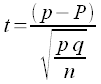
Note that the form is still (sample statistic - population parameter)/standard error for the statistic.
=(0.5625-0.51)/SQRT(0.5625*0.4375/32)
=0.5545
The t-statistic t does not exceed the t-critical value, so the difference is not statistically significant. We fail to reject the null hypothesis of no change.
The p-value is calculated as above using the absolute value of the t-statistic.
=TDIST(ABS(0.5545);32-1;2)
=0.58
The maximum level of confidence c we can have that this difference is significant is only 42%, far too low to say there is a difference.