Population: The complete group of measurements, observations, objects or people.
Sample: A part of the population. A sample is usually more than five measurements, observations, objects, or people, but always smaller than the complete group.
Examples
We could use the ratio of females to males to estimate the ratio of females to males on campus. Population: the College students. Sample: The class.
We could use the average body fat index for a randomly selected group of females on campus to determine the average body fat index for females in the FSM between the ages of 18 and 22. Population: Females in the FSM. Sample: those females on cmapus that we've measured.
Ways to gather statistics
Generalizing: The process of extending from sample results to population.
| Level of measurement | Definition | Examples |
|---|---|---|
| Nominal | In name only | Sorting by categories such as red, orange, yellow, green, blue, indigo, violet |
| Ordinal | In rank order, there exists an order but differences and ratios have no meaning | Grading systems: A, B, C, D, F Rating systems: ««««,«««,««,«, |
| Interval | Differences have meaning, but not ratios. There is either no zero or the zero has no mathematical meaning. | The numbering of the years: 2001, 2000, 1999. The year 2000 is 1000 years after 1000 A.D. (the difference has meaning), but it is NOT "twice as many years (the ratio has no meaning). Someone born in 1998 is eight years younger than someone born in 1990, but they are not half the age of someone born 999 A.D. |
| Ratio | Difference and ratios have meaning. There is a mathematically meaningful zero | Physical quantities: distance, height, speed, velocity, time in seconds, altitude, acceleration, mass. 100 kg is twice as heavy as 50 kg. Ten dollars is 1/10 of $100. |
Random samples
n: a variable that represents any number. Also the number of elements/objects/people in a sample. The sample size.
A simple random sample of n measurements from a population is one selected in a way that any member of the population is equally likely to be selected.
Ensuring that a sample is random is difficult. Suppose I want to study how many Pohnpeians own cars, would people I meet/poll on main street Kolonia be a random sample? Why? Why not?
Computers can generate pseudo-random numbers. Pseudo:falsely random. They are very close to random but are actually not necessarily random. We will look at computer generated random number later in the course. Useful in simulations, not in other situations.
Coins and dice can be used to generate random numbers.
To ensure a "balanced sample": Suppose I want to do a study of the average body fat of young people in the FSM. If I choose as my sample students a random sample of students at the national campus then I am likely to wind up with Pohnpeians being overrepresented. The national population is half Chuukese, but the campus population is more than half Pohnpeian. Hence I am likely, in a random selection of 100 students to pick too many Pohnpeians.
| State | Population | Fractional share of national population (relative frequency) | Number of student seats held by state at the national campus | Fractional share of the national campus student seats |
| Chuuk | 52870 | 0.50 | 679 | 0.20 |
| Kosrae | 7354 | 0.07 | 316 | 0.09 |
| Pohnpei | 33372 | 0.32 | 2122 | 0.62 |
| Yap | 11128 | 0.11 | 287 | 0.08 |
| 104724 | 1.00 | 3404 | 1.00 |
The solution is to use stratified sampling. First I decide I want 100 students that are representative of the four states. Then I can randomly pick 50 Chuukese students, 7 Kosraen, 32 Pohnpeian, and 11 Yapese and I will accurately reflect the makeup of the nation rather than the national campus. Each state would be considered a single "strata."
Used where a population is in some sequential order. A start point must be randomly chosen. Useful in a measuring a timed event. Never used if there is a cyclical or repetitive nature to a system: If sample rate » cycle rate then the results are not going to be randomly distributed measurements.
The population is divided into naturally occurring subunits and then subunits are randomly selected for measurement. In this method it is important that subunits (subgroups) are fairly interchangeable. If we want to poll the people in Kitti's opinion on whether they would pay for water if water was guaranteed to be clean and available 24 hours a day. We could cluster by breaking up the population by kosapw and then randomly choose a few kosapws and poll everyone in these kosapws. The results would probably be generalizable to all Kitti.
Convenience sampling
Results or data that are easily obtained is used. Highly unreliable as a method of getting a random samples. Often biased.
(P13-14 5,7) (P21-23 5, 13)
Using Excel to generate random numbers
Bar graphs are also called column charts. Use Excel to do your graphing. There is an example in the online spreadsheet. If a column chart is sorted so that the columns are in descending order, then it is called a Pareto Charts. Pareto charts are useful ways to convey rank order as well as numerical data.
Circle graphs ("pie" chart) Whole circle is 100% Used when data "adds" to a whole, e.g. state populations add to yield national population.
Line graph
xy graph. When you have two sets of continuous data (value versus value, no categories), use an xy graph. Often used in science
Histograms and Relative Frequency Distributions
Often used for interval or ratio level measurements. Not possible at nominal or ordinal level. Akin to a "bar graph" (column graph in Excel) but each "column" represents an interval that is the same for each and every column. The original data is gathered into sets or groups of data. Excel refers to this as putting the data into bins.
How to make a histogram
| Bin Upper Limits | Frequency |
| =min + bin width | =FREQUENCY(data,bins) |
| + bin width | |
| + bin width | |
| + bin width | |
| max |
For the female height data:
58, 58, 59.5, 59.5, 60, 60, 60, 60, 60, 61, 61, 61.2, 61.5, 62,
62, 62, 62, 62, 62, 62, 62, 62, 62, 62, 62, 63, 63, 63, 63.5,
64, 64, 64, 64, 65, 65, 66, 66
Five bins would produce the following results:
Min = 58
Max = 66
Range = 8
Width = 1.6
| Height CUL | Frequency |
|---|---|
| 59.6 | 4 |
| 61.2 | 8 |
| 62.8 | 13 |
| 64.4 | 8 |
| 66 | 4 |
| Sum: | 37 |
Note that 61.2 is INCLUDED in the bin that ends at 61.2. Excel includes the class upper limit.
There are quirks to the process of making charts in Microsoft Excel, and the quirks vary from version of Excel to version of Excel. This lab has Excel 95, Excel 97, and Excel 2000 present due to the varying ages of the computers. Because the quirks are version unique, moving from computer to computer will cause confusion as you move from version to version. Hence I recommend you sit at the same computer each day so as to become accustomed to the quirks of your particular version.
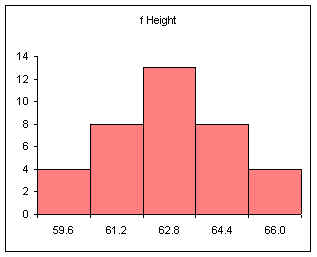
Note that the gap width on the columns has been set to zero.
Relative Frequency (also known as probability)
Divide each frequency by the sum to get the relative frequency
| Height CUL | Frequency | Relative Frequency f/n or P(x) |
|---|---|---|
| 59.6 | 4 | 0.11 |
| 61.2 | 8 | 0.22 |
| 62.8 | 13 | 0.35 |
| 64.4 | 8 | 0.22 |
| 66 | 4 | 0.11 |
| Sum: | 37 | 1.00 |
The relative frequency always adds to one (rounding causes the above to add to 1.01, if all the decimal places were used the relative frequencies would add to one.
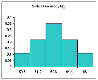
The area under the relative frequency columns is equal to one.
An in-class example from Fall 2001 with integers:
0, 1, 2, 2, 3, 3, 3, 4, 4, 4, 4.5, 5, 5, 5, 6, 6, 7, 8, 9, 10
Five bins
min = 0
max = 10
range = 10
width = 10/5 = 2
| Bin Num | Calculation | Bins | Frequency | Relative Frequency f/n or P(x) |
|---|---|---|---|---|
| 1 | min + width | 2 | 4 | 0.20 |
| 2 | + width | 4 | 6 | 0.30 |
| 3 | + width | 6 | 6 | 0.30 |
| 4 | + width | 8 | 2 | 0.10 |
| 5 | + width | 10 | 2 | 0.10 |
| Sum: | 20 | 1.00 |
Note that the above does not conform to either standard statistical practice nor to Brase and Brase. The above method is simply the easiest way to produce equal width bins and to conform to Microsoft Excel's inclusion of the class upper limit.
Homework Fall 2001: Using five bins, produce both a frequency histogram and a relative frequency histogram for the following 25 body fat percentages for females in MS 150 and MS 101 Summer and Fall 2001.
95, 112, 113, 116, 116, 117, 120, 123, 125, 125, 126, 126, 127, 127, 128, 130, 132, 132, 132, 134, 143, 147, 149, 152, 160.
See the BFI tab of the notebook statistics_fall2001.xls to see various shapes of histograms.