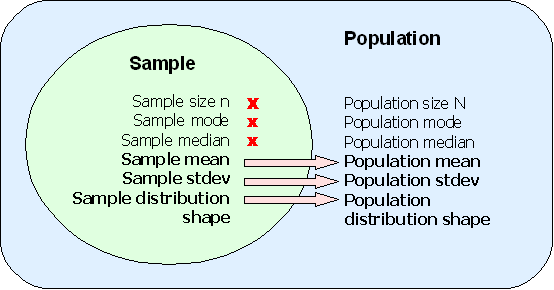
Whenever we use a single statistic to estimate a parameter we refer to the estimate as a point estimate for that parameter. When we use a statistic to estimate a parameter, the verb used is "to infer." We infer the population parameter from the sample statistic.
Some population parameters cannot be inferred from the statistic. The population size N cannot be inferred from the sample size n. The population minimum, maximum, and range cannot be inferred from the sample minimum, maximum, and range. Populations are more likely to have single outliers than a smaller random sample.
The population mode and median usually cannot be inferred from a smaller random sample. There are special circumstances under which a sample mode and median might be a good estimate of a population mode and median, these circumstances are not covered in this class.
The statistic we will focus on is the sample mean x. The normal distribution of sample means for many samples taken from a population provides a mathematical way to calculate a range in which we expect to "capture" the population mean and to state the level of confidence we have in that range's ability to capture the population mean µ.
The sample mean x is a point estimate for the population mean µ
The sample mean x for a random sample will not be the exact same value as the true population mean µ.
The error of a point estimate is the magnitude of estimate minus the actual parameter (where the magnitude is always positive). The error in using x for µ is ( x − µ ). Note that to take a positive value we need to use either the absolute value |( x - µ )| or √( x - µ )2.
Note that the error of an estimate is the distance of the statistic from the parameter.
Unfortunately, the whole reason we were using the sample mean x to estimate the population mean µ is because we did not know the population mean µ.
For example, given the mean body fat index (BFI) of 51 male students at the national campus is x = 19.9 with a sample standard deviation of sx = 7.7, what is the error |( x - µ )| if µ is the average BFI for male COMFSM students?
We cannot calculate this. We do not know µ! So we say x is a point estimate for µ. That would make the error equal to √(x − x)2 = zero. This is a silly and meaningless answer.
Is x really the exact value of µ for all the males at the national campus? No, the sample mean is not going to be the same as the true population mean.
The sample standard deviation sx is a reasonable point estimate for the population standard deviation σ. In more advanced statistics classes concern over bias in the sample standard deviation as an estimator for the population standard deviation is considered more carefully. In this class, and in many applications of statistics, the sample standard deviation sx is used as the point estimate for the population standard deviation σ.
We might be more accurate if we were to say that the mean µ is somewhere between two values. We could estimate a range for the population mean µ by going one standard error below the sample mean and one standard error above the sample mean. Remember, the standard error is the σ/√(n). Note that the formula for the standard error requires knowing the population standard deviation σ. We do not usually know this value. In fact, if we knew σ then we would probably also know the population mean µ. In section 9.2 we will use the sample standard deviation or sx/√(n) and the student's t-distribution to calculate a range in which we expect to find the population mean µ.
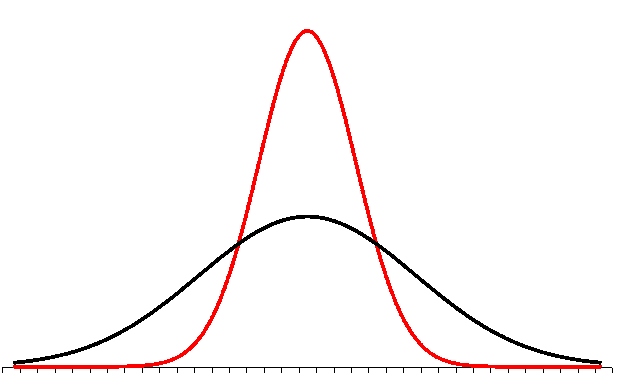
In the diagram the lower curve represents the distribution of data in a population with a normal distribution. Remember, distribution simply means the shape of the frequency or relative frequency histogram, now charted as a continuous line. The narrower and taller line is the distribution of all possible sample means from that population.
For the population curve (lower, broader) the distance to each inflection point is one standard deviation: ± σ. For the sample means (higher, narrower) the distance to each inflection point is one standard error of the mean: ± σ/√(n).
The area from minus one standard error to plus one standard error is still 68.2%.
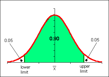
Here is a key point: If I set my estimate for µ to be between x - σ/√n and x + σ/√n, then there is a 0.682 probability that µ will be included in that interval.
The "68.2% probability" is termed "the level of confidence."
Probability note: the reality is that the population mean is either inside or outside the range we have calculated. We are right or wrong, 100% or 0%. Thus saying that there is a 68.2% probability that the population mean has been "captured" by the range is not actually correct. This is the main reason why we shift to calling the range for the mean a confidence interval. We start saying things such as "I am 68.2 percent confident the mean is in the range quoted." Statisticians assert that over the course of a lifetime, if one always uses a 68.2% confidence interval one will right 68.2% of the time in life. This is small comfort when an individual experimental result might be very important to you.
In many fields of inquiry a common level of confidence used is a 95% level of confidence. For the purposes of this course a 95% confidence interval is often used.

Note that when a confidence interval is not 95%, then specific reference to the chosen confidence level must be stated. Stating the level of confidence is always good form. While many studies are done at a 95% level of confidence, in some fields higher or lower levels of confidence may be common. Scientific studies often use 99% or higher levels of confidence.
There is always, however, a chance that one will be wrong. In Florida an election was "called" in favor of candidate Al Gore in the year 2000 in the United States based on a 99.5% level of confidence. Hours later the news organizations said George Bush had won Florida. A few hours later the news organizations would retract this second estimate and decide that the race was too close too call. The news organizations decided they had been wrong two times in row. Eventually a court case finally settled who had won the state of Florida. Even at a half a percent chance of being wrong one can still be wrong, even two times in a row.
When using the sample standard deviation sx to generate a confidence interval for the population mean, a distribution called the Student's t-distribution is used. The Student's t-distribution looks like the normal distribution, but the t-distribution changes shape slightly as the sample size n changes. The t-distribution looks like a normal distribution, but the shape "flattens" as n decreases. As the sample size decreases, the t-distribution becomes flatter and wider, spreading out the confidence interval and "pushing" the lower and upper limits away from the center. For n > 30 the Student's t-distribution is almost identical to the normal distribution. When we sketch the Student's t-distribution we draw the same heap shape with two inflection points.
To use the Student's t-distribution the sample must be a good, random sample. The sample size can be as small as n = 5. For n ≤ 10 the t-distribution will generate very large ranges for the population mean. The range can be so large that the estimate is without useful meaning. A basic rule in statistics is "the bigger the sample size, the better."
The spreadsheet function used to find limits from the Student's t-distribution does not calculate the lower and upper limits directly. The function calculates a value called "t-critical" which is written as tc. t-critical muliplied by the Standard Error of the mean SE will generate the margin of error for the mean E.
Do not confuse the standard error of the mean with the margin of error for the mean. The Standard Error of the mean is sx/√(n). The Margin of Error for the mean (E) is the distance from either end of the condifendence interval to the middle of the confidence interval. The margin of error is produced from the Standard Error:
Margin of Error for the mean = tc*standard error of the mean
Margin of Error for the mean = tc*sx/√n
The confidence interval will be:
x - E ≤ µ ≤ x + E
The t-critical valus will be calculated using the spreadsheet function TINV. TINV uses the area in the tails to calculate t-critical. The area under the whole curve is 100%, so the area in the tails is 100% − confidence level c. Remember that in decimal notation 100% is just 1. If the confidence level c is in decimal form use the spreadsheet function below to calculate tc:
=TINV(1−c,n−1)
If the confidence level c is entered as a percentage with the percent sign, then make sure the 1 is written as 100%:
=TINV(100%−c%,n−1)
The TINV function adjusts t-critical for the sample size n. The formula uses n − 1. This n − 1 is termed the "degrees of freedom." For confidence intervals of one variable the degrees of freedom are n − 1.
Runners run at a very regular and consistent pace. As a result, over a fixed distance a runner should be able to repeat their time consistently. While individual times over a given distance will vary slightly, the long term average should remain approximately the same. The average should remain within the 95% confidence interval.
For a sample size of n = 10 runs from the college in Palikir to Kolonia town, a runner has a sample mean x time of 61 minutes with a sample standard deviation sx of 7 minutes. Construct a 95% confidence interval for my population mean run time.
Step 1: Determine the basic sample statistics
sample size n = 10
sample mean x = 61
 [61 is also the point est. for the pop. mean µ]
sample standard deviation sx = 7

Step 2: Calculate degrees of freedom, tc, standard error SE
degrees of freedom = 10 - 1 = 9
tc =TINV(1-0.95,10-1) = 2.2622
Standard Error of the mean sx/√n = 7/sqrt(10) = 2.2136
Keeping four decimal places in intermediate calculations can help reduce rounding errors in calculations. Alternatively use a spreadsheet and cell references for all calculations.
Step 3: Determine margin of error E
Margin of error E for the mean
 = tc*sx/√n = (2.4469)*(7)/√10 = 5.01
Given that: x - E ≤ µ ≤ x + E, we can substitute the values for x and E to obtain the 95% confidence interval for the population mean µ:
Step 4: Calcuate the confidence interval for the mean
61 − 5.01 ≤ µ ≤ 61 + 5.01
    55.99 ≤ µ ≤ 66.01
I can be 95% confident that my population mean µ run time should be between 56 and 66 minutes.
| Jumps | ||||||||
|---|---|---|---|---|---|---|---|---|
| 102 | 66 | 42 | 22 | 24 | 107 | 8 | 26 | 111 |
| 79 | 61 | 45 | 43 | 10 | 17 | 20 | 45 | 105 |
| 68 | 69 | 79 | 13 | 11 | 34 | 58 | 40 | 213 |
On Thursday 08 November 2007 a jump rope contest was held at a local elementary school festival. Contestants jumped with their feet together, a double-foot jump. The data seen in the table is the number of jumps for twenty-seven female jumpers. Calculate a 95% confidence interval for the population mean number of jumps.
The sample mean x for the data is 56.22 with a sample standard deviation of 44.65. The sample size n is 27. You should try to make these calculations yourself. With those three numbers we can proceed to calculate the 95% confidence interval for the population mean µ:
Step 1: Determine the basic sample statistics
sample size n = 27
sample mean x = 56.22
sample standard deviation sx = 44.65

Step 2: Calculate degrees of freedom, tc, standard error SE
The degrees of freedom are n − 1 = 26
Therefore tcritical = TINV(1-0.95,27-1) = 2.0555
The Standard Error of the mean SE = sx/√27 = 8.5924

Step 3: Determine margin of error E
Therefore the Margin of error for the mean E
  tc* SE = 2.0555*8.5924 = 17.66
The 95% confidence interval for the mean is x − E ≤ µ ≤ x + E
Step 4: Calcuate the confidence interval for the mean
56.22 − 17.66 ≤ µ ≤ 56.22 + 17.66
        38.56 ≤ µ ≤ 73.88
The population mean for the jump rope jumpers is estimated to be between 38.56 and 73.88 jumps.
In 2003 a staffer at the Marshall Islands department of education noted in a newspaper article that Marshall's Island public school system was not the weakest in Micronesia. The staffer noted that Marshall's was second weakest, commenting that education metrics in the Marshall's outperform those in Chuuk's public schools.
In 2004 fifty students at Marshall Islands High School took the entrance test. Ten students Achieved admission to regular college programs. In Chuuk state 7% of the public high school students gain admission to the regular college programs. If the 95% confidence interval for the Marshall Islands proportion includes 7%, then the Marshallese students are not academically more capable than the Chuukese students, not statistically significantly so. If the 95% confidence interval does not include 7%, then the Marshallese students are statistically significantly stronger in their admissions rate.
Finding the 95% confidence interval for a proportion involves estimating the population proportion p. The fifty students at Marshall Islands High School are taked as a sample. The proportion who gained admission, 10/50 or 20%, is the sample proportion. The population proportion is treated as unknown, and the sample proportion is used as the point estimate for the population proportion.
Note: In this text the letter p is used for the sample proportion of successes instead of "p hat". A capital P is used to refer to the population proportion.
The letter n refers to the sample size. The letter p is the sample proportion of successes. The letter q is the sample proportion of failures. In the above example n is 50, p is 10/50 or 0.20, and q is 40/50 or 0.80
Estimating the population proportion P can only be done if the following conditions are met:
np > 5
nq > 5
In the example np = (50)(0.20) = 10 which is > 5. nq = (50)(0.80) = 40 which is also > 5
The standard error of a proportion is √(pq/n). For the example above the standard error is:
=sqrt((0.2)*(0.8)/50)
The standard error for the proportion is 0.0566. The margin of error E is then calculated in much the same way as in the section above, by multiplying tc by the standard error. tc is still found from the TINV function. The degrees of freedom will remain n-1.
The margin of error E = tc*√(pq/n)
=TINV(1-0.95,50-1)*sqrt((0.2)*(0.8)/50)
The margin of error E is 0.1137
The confidence interval for the population proportion P is:
p − E ≤ P ≤ p + E
0.20 − 0.1137 ≤ P ≤ 0.20 + 0.1137
0.0863 ≤ P ≤ 0.3137
The result is that the expected population mean for Marshall Island High School is between 8.6% and 31.2%. The 95% confidence interval does not include the 7% rate of the Chuuk public high schools. While the college entrance test is not a measure of overall academic capability, there are few common measures that can be used across the two nations. The result does not contradict the staffer's assertion that MIHS outperformed the Chuuk public high schools. This lack of contradiction acts as support for the original statement that MIHS outperformed the public high schools of Chuuk in 2004.
Homework: In twelve sumo matches Hakuho bested Tochiazuma seven times. What is the 90% confidence interval for the population proportion of wins by Hakuho over Tochiazuma. Does the interval extend below 50%? A commentator noted that Tochiazuma is not evenly matched. If the interval includes 50%, however, then we cannot rule out the possibility that the two-win margin is random and that the rikishi (wrestlers) are indeed evenly matched.
Hakuho won that night, upping the ratio to 8 wins to 5 losses to Tochiazuma. Is Hakuho now statistically more likely to win or could they still be evenly matched at a confidence level of 90%?
Suppose you are designing a study and you have in mind a particular error E you do not want to exceed. You can determine the sample size n you'll need if you have prior knowledge of the standard deviation sx. How would you know the sample standard deviation in advance of the study? One way is to do a small "pre-study" to obtain an estimate of the standard deviation. These are often called "pilot studies."
If we have an estimate of the standard deviation, then we can estimate the sample size needed to obtain the desired error E.
Since E = tc*sx/√n, then solving for n yields = (tc*sx/E)²
Note that this is not a proper mathematical solution because tc is also dependent on n. While many texts use zc from the normal distribution in the formula, we have not learned to calculate zc.
In the "real world" what often happens is that a result is found to not be statistically significant as the result of an initial study. Statistical significance will be covered in more detail later. The researchers may have gotten "close" to statistical significance and wish to shrink the confidence interval by increasing the sample size. A larger sample size means a smaller standard error (n is in the denominator!) and this in turn yields a smaller margin of error E. The question is how big a sample would be needed to get a particular margin of error E.
The value for tc from pilot study can be used to estimate the new sample size n. The resulting sample size n will be slightly overestimated versus the traditional calculation made with the normal distribution. This overestimate, while slightly unorthodox, provides some assurance that the error E will indeed shrink as much as needed.
In a study of body fat for 51 males students a sample mean x of 19.9 with a standard deviation of 7.7 was measured. This led to a margin of error E of 2.17 and a confidence interval 17.73 ≤ µ ≤ 22.07
Suppose we want a margin of error E = 1.0 at a confidence level of 0.95 in this study of male student body fat. We can use the sx from the sample of 51 students to estimate my necessary sample size:
n = (2.0086*7.7/1)2 = 239.19 or 239 students. Thus I estimate that I will need 239 male students to reduce my margin of error E to ±1 in my body fat study.
Other texts which use zc would obtain the result of 227.77 or 228 students. The eleven additional students would provide assurance that the margin of error E does fall to 1.0.
That one can calculate a sample size n necessary to reduce a margin of error E to a particular level means that for any hypothesis test (chapter ten) in which the means have a mathematical difference, statistical significance can be eventually be attained by sufficiently increasing the sample size. This may sound appealing to the researcher trying to prove a difference exists, but philosophically it leaves open the concept that all things can be proven true for sufficiently large samples.