As noted in earlier chapters, statistics are the measures of a sample. The measures are used to characterize the sample and to infer measures of the population termed parameters.
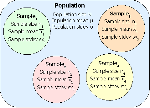
A parameter is a numerical description of a population. Examples include the population mean μ and the population standard deviation σ.
A statistic is a numerical description of a sample. Examples include a sample mean x and the sample standard deviation sx.
Good samples are random samples where any member of the population is equally likely to be selected and any sample of any size n is equally likely to be selected. Consider four samples selected from a population. The samples need not be mutually exclusive as shown, they may include elements of other samples.
The sample means x1, x2, x3, x4, can include a smallest sample mean and a largest sample mean. Choosing a number of bins can generate a histogram for the sample means. The question this chapter answers is whether the shape of the distribution of sample means from a population is any shape or a specific shape.
The shape of the distribution of the sample mean is not any possible shape. The shape of the distribution of the sample mean, at least for good random samples with a sample size larger than 30, is a normal distribution. That is, if you take random samples of 30 or more elements from a population, calculate the sample mean, and then create a relative frequency distribution for the means, the resulting distribution will be normal.
In the following diagram the underlying data is bimodal and is depicted by the columns with thin outlines. Thirty data elements were sampled forty times and forty sample means were calculated. A relative frequency histogram of the sample means is plotted with a heavy black outline. Note that though the underlying distribution is bimodal, the distribution of the forty means is heaped and close to symmetrical. The distribution of the forty sample means is normal.
The center of the distribution of the sample means is, theoretically, the population mean. To put this another simpler way, the average of the sample averages is the population mean. Actually, the average of the sample averages approaches the population mean as the number of sample averages approaches infinity.
The sample mean distribution is a heap shaped, as in the shape of the normal distribution, and centered on the population mean.
If the sample size is 30 or more, then the sample means are NORMALLY distributed even when the underlying data is NOT normally distributed! If the sample size is less than 30, then the distribution of the samples means is normal if and only if the underlying data is normally distributed.
The normal distribution of the sample means (averages) allows us to use our normal distribution probabilities to estimate a range for μ. The mean of the sample means is a point estimate for the population mean μ.
The mean of the sample means can be written as:
![]()
In this text the above is sometimes written as μ x
The value of the mean of the sample means μ x is, for a very large number of samples each of which has a very large sample size, the population mean. As a practical matter we use the mean of a single large sample. How large? The sample size must be at least n = 30 in order for the sample mean (a statistic) to be a good estimate for the population mean (a parameter). This requirement is necessary to ensure that the distribution of the sample means will be normal even when the underlying data is not normal. If we are certain the data is normally distributed, then a sample size n of less than 30 is acceptable.
Later in the course we will modify the normal distribution to handle samples of sizes less than 30 for which the distribution of the underlying data is either unknown or not normal. This modification will be called the student's t-distribution. The student's t-distribution is also heap-shaped.
The normal distribution, and later the student's t-distribution, will be used to quote a range of possible values for a population mean based on a single sample mean. Knowing that the sample mean comes from a heap-shaped distribution of all possible means, we will center the normal distribution at the sample mean and then use the area under the curve to estimate the probability (confidence) that we have "captured" the population mean in that range.
The Central Limit Theorem is the theory that says "for increasingly large sample sizes n, the sample mean approaches ever closer the population mean."
There is one complication: the sample standard deviation of a single sample is not a good estimate of the standard deviation of the sample means. Note that the distribution of the sample means is NARROWER than the sample in the above example. The shape of the distribution of the sample means is narrower and taller than the shape of the underlying data. In the diagram, the shape of the underlying data is normal, the taller narrower distribution is the distribution of all the sample means for all possible samples.
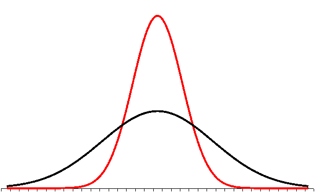
The standard deviation of a single sample has to be reduced to reflect this. This reduction turns out to be inversely related to the square root of the sample size. This is not proven here in this text.
The standard deviation of the distribution of the sample means is equal to the actual population standard deviation divided by the square root of n.
The standard deviation divided by the square root of the sample size is called the standard error of the mean.
If σ is known, then the above formula can be used and the distribution of the sample mean is normal.
As a practical matter, since we rarely know the population standard deviation σ, we will use the sample standard deviation sx in class to estimate the standard deviation of the sample means. This formula will then appear in various permutations in formulas used to estimate a population mean from a sample mean. When we use the sample standard deviation sx we will use the student's t-distribution. The student's t-distribution looks like a normal distribution. The student's t-distribution, however, is adjusted to be a more accurate predictor of the range for a population mean. Later we will learn to use the student's t-distribution. Until that time we will play a little fast and loose and use sample standard deviations to calculate the standard error of the mean.