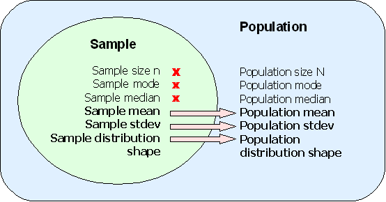
Inferential statistics is all about measuring a sample and then using those values to predict the values for a population. The measurements of the sample are called statistics, the measurements of the population are called parameters. Some sample statistics are good predictors of their corresponding population parameter. Other sample statistics are not able to predict their population parameter.
The sample size will always be smaller than the population. The population size N cannot be predicted from the sample size n. The sample mode is not usually the same as the population mode. The sample median is also not necessarily a good predictor of the population median.
The sample mean for a good, random sample, is a good point estimate of the population mean μ. The sample standard deviation sx predicts the population standard deviation σ. The shape of the distribution of the sample is a good predictor of the shape of the distribution of the population.
That the shape of the population distribution can be predicted by the shape of the distribution of a good random sample is important. Later in the course we will be predicting the population mean μ. Instead of predicting a single value we will predict a range in which the population mean will likely be found.
Consider as an example the following question, "How long does it take to drive from Kolonia to the national campus on Pohnpei?" A typical answer would be "Ten to twenty minutes." Everyone knows that the time varies, so a range is quoted. The average time to drive to the national campus is somewhere in that range.
Determining the appropriate range in which a population mean will be found depends on the shape of the distribution. A bimodal distribution is likely to need a larger range than a symmetrical bell shaped distribution in order to be sure to capture the population mean.
As a result of the above, we need to understand the shape of distributions generated by different systems. The most important shape in statistics is the shape of a purely random distribution, like that generated by tossing many pennies.
In class exercise: flipping seven pennies. Student flip seven pennies and record the number of heads. The data for a section is gathered and tabulated. The students then prepare a relative frequency histogram of the number of heads and calculate the mean number of heads from Σ x*p(x).
In the table below, seven pennies are tossed eight hundred and fifty eight times. For each toss of the seven pennies, the number of pennies landing heads up are counted.
| # of heads x | Frequency | Rel Freq P(x) |
|---|---|---|
| 7 | 9 | 0.0105 |
| 6 | 112 | 0.1305 |
| 5 | 147 | 0.1713 |
| 4 | 228 | 0.2657 |
| 3 | 195 | 0.2273 |
| 2 | 120 | 0.1399 |
| 1 | 45 | 0.0524 |
| 0 | 2 | 0.0023 |
| 858 | 1.00 |
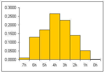
The relative frequency histogram for a large number of pennies is usually a heap-like shape. For seven pennies the theoretic shape of an infinite number of tosses can be calculated by considering the whole sample space for seven pennies
HHHHHHH HHHHHHT HHHHHHTT HHHHTTT HHHTTTT HHTTTTTT HTTTTTT TTTTTTT
        HHHHHTH HHHHHTHT HHHTHTT HHTHTTT THTTTTTH TTTTTTH
        HHHHTHH HHHHTHHT HHTHHTT HTHHTTT THTTTTHT TTTTTHT
          ...     ...       ...    ...      ...     ...
If one works out all the possible combinations then one attains:
(two sides)^(7 pennies) = 128 total possibilities
1 way to get seven heads/128 total possible outcomes = 1/128= 0.0078
7 ways to get six heads and one tail/128 possibilities = 7/128 =0.0547
21 ways to get five heads and two tails/128 = 21/128 = 0.1641
35 ways to get four heads and three tails/128 = 35/128 = 0.2734
35 ways to get three heads and four tails/128 = 35/128 = 0.2734
21 ways to get two heads and five tails/128 = 21/128 = 0.1641
7 ways to get one head and six tails/128 possibilities = 7/128 =0.0547
1 way to get seven tails/128 total possible outcomes = 1/128= 0.0078
If the theoretic relative frequencies (probabilities) are added to our table:
| # of heads x | Frequency | Rel Freq P(x) | Theoretic |
|---|---|---|---|
| 7 | 9 | 0.0105 | 0.0078 |
| 6 | 112 | 0.1305 | 0.0547 |
| 5 | 147 | 0.1713 | 0.1641 |
| 4 | 228 | 0.2657 | 0.2734 |
| 3 | 195 | 0.2273 | 0.2734 |
| 2 | 120 | 0.1399 | 0.1641 |
| 1 | 45 | 0.0524 | 0.0547 |
| 0 | 2 | 0.0023 | 0.0078 |
| 858 | 1.00 | 1.00 |
If the theoretic relative frequencies are added as a line to our graph, the following graph results:
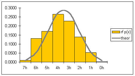
The gray line represents the shape of the distribution for an infinite number of coin tosses. The shape of the distribution is symmetrical.
If both the number of pennies is increased as well as the number of tosses, then the graph would become smoother and increasingly symmetrical. Below is a graph for tens of thousands of tosses of 21 pennies.
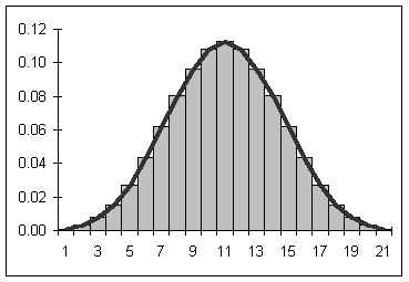
If the number of pennies and tosses are both allowed to go to infinity, then a smooth curve results looking a lot like the curve seen above. The smooth curve that results can be described by a function. Statistical mathematicians would say that as the number of sides and tosses approaches infinity, the discrete distribution approaches a continuous distribution described by the function below.

In the above function, σ is the population standard deviation, μ is the population mean, e is the base e, and π is pi. The name of this function is the "normal" curve. I like to think of it as being called normal because it is what "normally" happens if you toss a lot of pennies a lot of times! If the above function is graphed for a mean μ = 0 and a population standard deviation σ = 1, then the following graph results:
The above function has the following properties:
The area under each "section" of the normal curve can be seen in the following diagram.
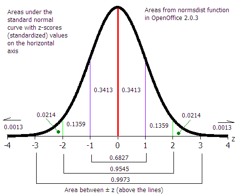
For example, the area under the curve beyond (to the right of) μ + 2σ is 0.0228 or 2.28%. The probability of a data value being greater than μ + 2σ is 0.0228. A data value could be expected out here once in about 44 instances.
6σ: "Six sigma" A business quality program that attempts to bring error down to 3 in a million (μ + 6σ)
The shape of the normal curve is affected by the standard deviation. In the diagram below m is the mean μ and sx is the standard deviation.
Changes to the mean shift the normal curve horizontally:
Let us begin with a more familiar example from our work earlier in the term.
Heap like shapes often result from histograms of data. The following is a frequency table for the height data for 60 females in statistics class in an earlier term.
| Female height CUL | Frequency | Relative Frequency |
|---|---|---|
| 59.6 | 6 | 0.10 |
| 61.2 | 16 | 0.27 |
| 62.8 | 18 | 0.30 |
| 64.4 | 16 | 0.27 |
| 66 | 4 | 0.07 |
| Sums: | 60 | 1.00 |
The following relative frequency histogram for the heights of 60 females above has the following distribution:
Imagine changing this discrete distribution into a continuous distribution.
The probability distribution above says that 10% of the women are less than or equal to 59.6 inches tall. 27% of the women measured are taller than 59.6 inches and shorter than or equal to 61.2 inches. What is the probability of finding a female student taller than 64.4 inches tall? Seven percent. The area "under" each segment of the "curve" is the probability of a women being in that range of heights.
The difficulty with the above analysis is seen in attempting to answer the following question: What percentage of female students are taller than 60 inches? This cannot easily be determined from the above data. An answer could be interpolated, but that would be the best we would be able to do.
In some instances the actual shape of the population distribution is not exactly known, but the distribution is expected to be heaped, to behave "normally" and heap up in the manner of the normal distribution.
Because there is a mathematical equation for the normal distribution, the probabilities (the areas under the curve!) can be determined mathematically.
Suppose we know that sixty customers arrive at a sakau market on a Friday night at a mean time of μ = 7:00 P.M. with a standard deviation of σ = 30 minutes (0.5 hours). Suppose also that the time of arrival for the customers is normally distributed (note that areas are rounded).
Note that in the above example the population mean μ and population standard deviation σ are used. Our normal distribution work is based on a theories that use the population parameters. Later in the course we will use a modified normal distribution called the student's t-distribution to work with sample statistics such as the sample mean x and the sample standard deviation sx for small samples. For many examples in this text, the population parameters are not known. Until the student's t-distribution is introduced, data that forms a reasonably "heap-like" shape will be analyzed using the normal distribution.
The probability p is the same as the area under the normal curve. Probability, expressed often as a percentage, is area. Probability is also the relative frequency. In this class probability, p, area, and relative frequency are all used interchangeably.
If x is not an whole number of standard deviations from the mean, then we cannot use a diagram as seen above. Spreadsheets have a function that calculates the area (probability) to the left of ANY x value. The letter p for probability is used for the area to the left of x.
The function that calculates the area to the left of x is:
=normdist(x,μ,σ,1)
Note that OpenOffice.org on Windows uses semi-colons where commas appear in the formula above. When in doubt, if a multi-argument formula generates an error and the values are all correct, try semi-colons.
The mean height μ for 43 female students in statistics is 62.0 inches with a standard deviation of 1.9. Determine the probability that a student is less than 60 inches tall (five feet tall).
In OpenOffice the probability p =
=normdist(60,62,1.9,1)
=0.1463
14.63% of the area is to the left of 60 inches. The probability a female student in statistics class is below 60 inches is 14.63%.
Notation note: In probability notation the above would be written p(x < 60) = 0.1463
When the words "less than, smaller, shorter, fewer, up to and including" are used then the NORMDIST function can be used to calculate the probability.
The mean number of cups of sakau consumed in sakau markets on Pohnpei is μ = 3.65 with a standard deviation of σ = 2.52. Note that this data is actually based on customer data for 227 customers at four markets - one near Kolonia and three in Kitti. Although this data is actually sample data and not population data, we will treat the mean and standard deviation as population parameters. The data is not perfectly normally distributed. The data is, however, distributed in a reasonably smooth heap.
What is the probability a customer will drink more than five cups?
Note the word "more." If the question were "What is the probability that a customer will drink less than five cups, then the solution would be =NORMDIST(5,3.65,2.52,1). This result is 0.70 or a 70% probability a customer will drink less than five cups.
The area under the whole normal curve is 1.00. Remember that 1.00 is also 100%. If 70% drink less than five cups, then we can calculate the probability that those who drink more than five cups is 30%. 100% − 70% = 30%.
Or 1.00 − 0.70 = 0.30
Making a sketch of the normal curve including the mean, the x-value, and the area of interest can help determine when to subtract a result from one and when to not.
A study of the prevalence of diabetes in a village on Pohnpei found a mean fasting blood sugar level of μ = 117 with a standard deviation σ = 33 in mg/dl for females aged 20 to 29 years old. Blood sugar levels between 120 and 130 are considered borderline diabetes cases. What percentage of the females aged 20 to 29 years old in this village are between a mean fasting blood sugar of 120 and 130 mg/dl?
For this example, presume that the distribution is normal.
The probability is the percentage. The probability is the area between x = 120 and x = 130 as seen in the image below.
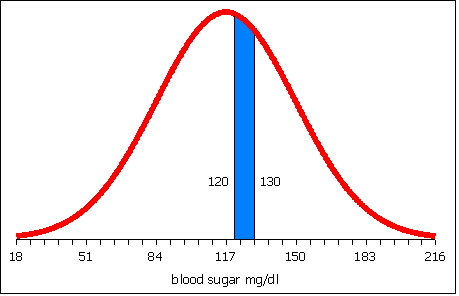
In probability notation this would be written p(120 < x < 130) = ?
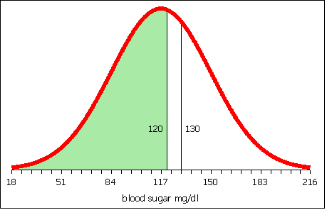
To obtain the area between 120 and 130, calculate the area to the left of 120.
Then calculate the area to the left of 130.
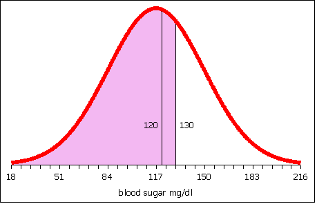
Subtract the area to the left of 120 from the area to the left of 130. What remains is the area between 120 and 130.
The table below represents a spreadsheet laid out to calculate the area to the left of 120 in column B and the area to the left of 130 in column C.
| A | B | C | D | |
|---|---|---|---|---|
| 1 | x | 120 | 130 | |
| 2 | mean μ | 117 | 117 | |
| 3 | stdev σ | 33 | 33 | |
| 4 | normdist | =NORMDIST(B1,B2,B3,1) | =NORMDIST(C1,C2,C3,1) | =C4-B4 |
| 4 | normdist | 0.54 | 0.65 | 0.11 |
Row four is presented twice: once with the formulas and once with the results of the formulas.
The area to the left of 120 is 0.54. The area to the left of 130 is 0.65. 0.65 − 0.54 is 0.11. The probability that females aged 20 to 29 years old in this village have a blood sugar level between 120 and 130 is 11%.
Conversely, given a probability, a mean, and a standard deviation, an x value can be calculated.
On the college essay admissions test a perfect score is 40. In a recent spring run of the admissions test the mean score was 21 and the standard deviation was 12. Below what score x are the lowest 33% of the student scores? Presume that the data is normally distributed.
In this case we have an area. Percentages are probabilities. Probabilities are area under the curve. We do not know x. To find the area to the left of x the function NORMINV is used. The letter p is the probability, the area.
=NORMINV(p,μ,σ)
In this case area =NORMINV(0.33,21,12). Note that the area is expressed as a decimal. Alternatively the area could be entered as 33%. The result of this calculation is 15.72. 33% of the students scored below a 15.72 on the essay test.

Suppose the height of women at the College is normally distributed with a mean of 62.0 inches and a standard deviation of 1.9 inches. Suppose I want to know the minimum height of the top 10% of the female students at the College.
In this instance I have a probability, the top 10%. The NORMINV function, however, requires the area to the right of x. If the area to the right is 10%, then the area to the left is 100% − 10% = 90%.
area =NORMINV(0.90,62,1.9)
The result is 64.43.
Thus the minimum height of the top 10% is 64.43 inches. If there are 350 women at the college, then 0.10 * 350 = 35 women can be expected to be taller than 64.4 inches.
Domino's pizza knows that the average length of time from receiving an order to delivering to the customer is 20 minutes with a standard deviation 7 min 45 seconds. Treat these sample statistics as population parameters for now. Dominoes wants to guarantee a delivery time as part of a marketing campaign, "Your pizza in ___ minutes of your money back!" Dominoes is willing to refund 10% of their orders, what is the quickest delivery time they should set the grantee at?
The area to the left of x is 90% therefore the correct function is =NORMINV(0.9,20,7.75)
The result is 29.92 minutes
So you guarantee delivery in 30 minutes or less and you'll only pay out on 10% of the pizzas. (From another perspective this is a "Buy ten to get one free program").