Objective: Introduce students to systems that result in a linear equation and in a quadratic equation. Learn to use resulting equations to predict future positions. Do this in a manner which minimized the equipment necessary.
Materials: Timers, golf balls or other spherical objects. Timers can be stopwatches found built into many digital watches.
Courses: Usable in both MS 098 Transition to Algebra and MS 100 College Algebra. Can be also be used in cognitive approach courses
Lacking air tables, spark tape, air rail cars, laboratory stopwatches, or other typical equipment, the lab below sought to generate linear and quadratic equations from the least amount of equipment. These two laboratories exemplify some of the approach used in the cognitive approach: moving from a concrete system to an abstract mathematical system. Work spirals up from basic measurement (laying out the course) to algebra.
The golf ball is rolled across a level parking lot or other long smooth surface. Velocity should be reasonably fast to cover the distance. We opted to work in feet as that was the only unit of measurement available to us on the tape measure we possessed.
Students are placed every ten feet, if possible, and time the ball as it passes their position. The ball bowler has to release accurately at the zero line and call out their release so that the timers can start their stopwatches at the same time.
Many students will need instruction in the use of their digital wristwatches if these are used as timers. The bowler may need a couple of practice throws to find a velocity that is fairly steady. The ground should be level. The class found that our asphalt often caused the golf ball to bounce errantly and the students who were not timing decided to take up defensive positions to protect cars in the lot from the golf ball.
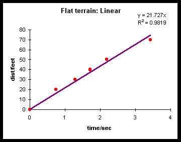
After the data is collected, a table of results is generated in the classroom. Note that in the example below timers were not present at ten and sixty feet.
| time/sec | dist/feet |
|---|---|
| 0 | 0 |
| 10 | |
| 0.74 | 20 |
| 1.28 | 30 |
| 1.72 | 40 |
| 2.19 | 50 |
| 60 | |
| 3.43 | 70 |
The students made an initial graph on their own paper of their results. Due to a lack of graph paper, two sheets of notebook paper were used. The lower sheet was turned at 90° to the upper sheet to create crude but effective graph paper. Students worked in small groups on their graphs while the instructor circulated in the classroom.
These results were later graphed by the students using Microsoft Excel. Due to the limited amount of computer laboratory space, the graphs were assigned as homework. A handout covered how to make a graph with Excel and how to insert a best fit trendline with the intercept set to zero. The options tab provided the equation of the line. The students did not in their work add in R², that is reported here only to illustrate the goodness of the fit. Despite bouncing erratically, the results are quite linear. The instructor was then present during the open laboratory hours to assist students with their graphs.
The best fit trendline then gave the class the equation of the line. The students, working again in small groups, were asked to work out the answers to questions such as how far the golf ball would go in ten seconds, the time it would take to cover one hundred feet, and so forth.
Without Excel, students could draw in a best fit line, determine the slope, and use this to make their predictions.
The above laboratory is repeated, but this time the golf ball is released from rest on a smooth constant slope. This was done on a different day than the above laboratory and timers were present for all seven timing positions. Students were also assigned to release and catch duties. The number of timers limited us to a single set of data. With more timers (and golf balls) teams of nine students could each do a data set.
A few trial runs were done to practice the starting and stopping of various digital watches.
The data was then recorded on the white board back in the classroom.
| time/sec | dist/feet |
|---|---|
| 0 | 0 |
| 4.56 | 10 |
| 6.57 | 20 |
| 8.14 | 30 |
| 9.48 | 40 |
| 10.65 | 50 |
| 11.85 | 60 |
| 12.46 | 70 |
Once again the students worked in teams of two to three to graph their data in class. This time the data did not appear to follow a straight line. Despite the crude method of collection, a quadratic curve resulted from the data.
As homework, the students graphed their results with Excel and then added both linear and quadratic trendlines. The students needed help with the quadratic trendline, Excel refers to this as a polynomial trendline with an order of 2. R² is again included only for reference in the graph below. The intercept was forced to be zero in the trendlines.
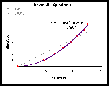
The equation can now be used to predict the position of the ball at various distances. In our situation we could predict the time at one hundred feet and then go back out and rerun the experiment with a timer at one hundred feet. This is what we did, with the result confirming our prediction. We were fortunate to have one hundred feet of constant slope on our driveway. Unfortunately the same could not be done for the thrown golf ball in the first laboratory.
If Excel is not available, then there a couple of options. One is to calculate the velocities for each leg - this will require a calculator:
| time (sec) | dist (feet) | velocity (feet/sec) |
|---|---|---|
| 0 | 0 | 0 |
| 4.56 | 10 | 2.19 |
| 6.57 | 20 | 4.98 |
| 8.14 | 30 | 6.37 |
| 9.48 | 40 | 7.47 |
| 10.65 | 50 | 8.55 |
| 11.85 | 60 | 8.33 |
| 12.46 | 70 | 16.39 |
The velocity can be graphed versus the time and then a best fit line can be drawn in and used to obtain the slope. This result is presented below:
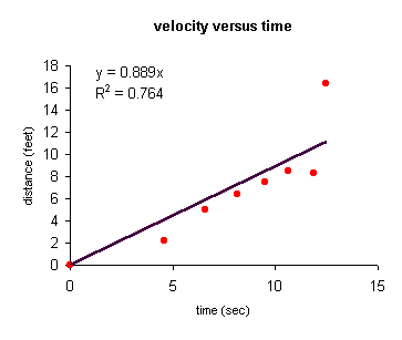
The equation for the quadratic is ½(0.889)x² or y = 0.445x². Another alternative is to calculate the changes in velocity with respect to time:
| time (sec) | distance (feet) | velocity (feet/sec) | acceleration (feet/sec2) |
| 0 | 0 | 0 | |
| 4.56 | 10 | 2.19 | 0.48 |
| 6.57 | 20 | 4.98 | 1.38 |
| 8.14 | 30 | 6.37 | 0.89 |
| 9.48 | 40 | 7.46 | 0.82 |
| 10.65 | 50 | 8.55 | 0.93 |
| 11.85 | 60 | 8.33 | -0.18 |
| 12.46 | 70 | 16.39 | 13.21 |
| Average: | 2.50 | ||
| Median: | 0.89 |
Note that the average acceleration is very sensitive to potential outliers in the data. Note that the median acceleration is a better measure as it reduces the impact of outliers. From the above table we would obtain ½(0.89)x² or y = 0.45x².
Although the above might be workable in SC 240 Physics, calculating the velocity and acceleration is too complex for MS 098 Transition to Algebra students. If we lacked Excel to produce the best fit quadratic equation, then I suggest obtaining the coefficient by using the end point to solve 70 = n(12.46)² to determine n = 0.45. Note that result is the same despite the data point being potentially errant. This procedure is lot more transparent than the above which borders on calculus.
Title III Math/Science Software Specialist
College of Micronesia-FSM
Developed by Dana Lee Ling with the support and funding of a U.S. Department of Education Title III grant and the support of the College of Micronesia - FSM. Notebook material ©1999 College of Micronesia - FSM. For further information on this project, contact dleeling@comfsm.fm Designed and run on Micron Millenia P5 - 133 MHz with 32 MB RAM, Windows 95 OS.