Seven Pennies Normal curve equation How continuous curves are used to determine probabilities Standardized or z-values Probability for any z
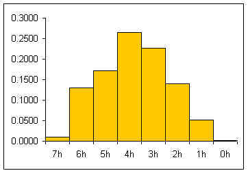
In the table below, seven pennies are tossed eight hundred and fifty eight times. For each toss of the seven pennies, the number of pennies landing heads up are counted.
| # of heads x |
Frequency | Rel Freq P(x) |
|---|---|---|
| 7 | 9 | 0.0105 |
| 6 | 112 | 0.1305 |
| 5 | 147 | 0.1713 |
| 4 | 228 | 0.2657 |
| 3 | 195 | 0.2273 |
| 2 | 120 | 0.1399 |
| 1 | 45 | 0.0524 |
| 0 | 2 | 0.0023 |
| 858 | 1.00 |
The relative frequency histogram for a large number of pennies is usually a heap-like shape. For seven pennies the theoretic shape of an infinite number of tosses can be calculated by considering the whole sample space for seven pennies
HHHHHHH HHHHHHT HHHHHHTT HHHHTTT HHHTTTT HHTTTTTT HTTTTTT TTTTTTT
        HHHHHTH HHHHHTHT HHHTHTT HHTHTTT THTTTTTH TTTTTTH
        HHHHTHH HHHHTHHT HHTHHTT HTHHTTT THTTTTHT TTTTTHT
          ...     ...       ...    ...      ...     ...
If one works out all the possible combinations then one attains:
(two sides)^(7 pennies) = 128 total possibilities
1 way to get seven heads/128 total possible outcomes = 1/128= 0.0078
7 ways to get six heads and one tail/128 possibilities = 7/128 =0.0547
21 ways to get five heads and two tails/128 = 21/128 = 0.1641
35 ways to get four heads and three tails/128 = 35/128 = 0.2734
35 ways to get three heads and four tails/128 = 35/128 = 0.2734
21 ways to get two heads and five tails/128 = 21/128 = 0.1641
7 ways to get one head and six tails/128 possibilities = 7/128 =0.0547
1 way to get seven tails/128 total possible outcomes = 1/128= 0.0078
If the theoretic relative frequencies (probabilities) are added to our table:
| # of heads x |
Frequency | Rel Freq P(x) |
Theoretic |
|---|---|---|---|
| 7 | 9 | 0.0105 | 0.0078 |
| 6 | 112 | 0.1305 | 0.0547 |
| 5 | 147 | 0.1713 | 0.1641 |
| 4 | 228 | 0.2657 | 0.2734 |
| 3 | 195 | 0.2273 | 0.2734 |
| 2 | 120 | 0.1399 | 0.1641 |
| 1 | 45 | 0.0524 | 0.0547 |
| 0 | 2 | 0.0023 | 0.0078 |
| 858 | 1.00 | 1.00 |
If the theoretic relative frequencies are added as a line to our graph, the following graph results:
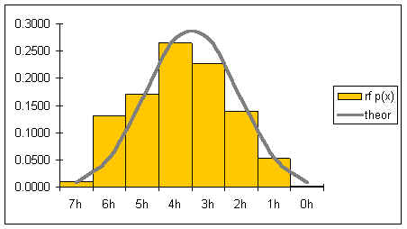
The gray line represents the shape of the distribution for an infinite number of coin
tosses. The shape of the distribution is symmetrical.
If both the number of pennies is increased as well as the number of tosses, then the graph
would become smoother and increasingly symmetrical. Below is a graph for tens of thousands
of tosses of 21 pennies.
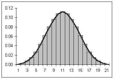
If the number of pennies and tosses are both allowed to go to infinity, then a smooth curve results looking a lot like the curve seen above. The smooth curve that results can be described by a function. Statistical mathematicians would say that as the number of sides and tosses approaches infinity, the discrete distribution approaches a continuous distribution descibed by the function below.
In the above function, s is the population standard deviation, m is the population mean, e is the base e, and p is pi. The name of this function is the "normal" curve. I like to think of it as being called normal because it is what "normally" happens if you toss a lot of pennies a lot of times! If the above function is graphed for a mean m = 0 and a population standard deviation s = 1, then the following graph results:
The above function has the following properties:
The area under each "section" of the normal curve can be seen in the following diagram.
For example, the area under the curve beyond (to the right of) m + 2s is 0.0215 or 2.15%. The probability of a data value being greater than m + 2s is 0.0215. A data value could be expected out here once in about 47 instances.
6s: "Six sigma" A business quality program that attempts to bring error role to 3 in a million (m + 6s)
The shape of the normal curve is affected by the standard deviation. In the diagram below m is the mean m and sx is the standard deviation.
Changes to the mean shift the normal curve horizontally:
Let me begin with a more familiar example from our work earlier in the term.
Heap like shapes often result from histograms of data. The following is a frequency table for the height data for 60 females at the College of Micronesia-FSM.
| Female height CUL | Frequency | Relative Frequency |
|---|---|---|
| 59.6 | 6 | 0.10 |
| 61.2 | 16 | 0.27 |
| 62.8 | 18 | 0.30 |
| 64.4 | 16 | 0.27 |
| 66 | 4 | 0.07 |
Sums: |
60 | 1.00 |
The following relative frequency histogram for the heights of 43 females at the College has the following distribution:
Imagine metamorphasizing this discrete distribution into a continous distribution.
The probability distribution above says that 10% of the women are less than or equal to 59.6 inches tall. 27% of the women measured are taller than 59.6 inches and shorter than or equal to 61.2 inches. What is the probability of finding a female student taller than 64.4 inches tall? Seven percent.
The difficulty with the above analysis is seen in attempting to answer the following question: What percentage of female students are taller than 60 inches? This cannot easily be determined from the above data. An answer could be interpolated, but that would be the best we would be able to do.
In some instances the actual shape of the population distribution is not exactly known, but the distribution is expected to be heaped, to behave "normally" and heap up in the manner of the normal distribution.
Because there is a mathematical equation for the normal distribution, the probabilities (the areas under the curve!) can be determined mathematically.
Suppose we know that sixty customers arrive at a sakau market on a Friday night at a mean time of 7:00 P.M. with a standard deviation of 30 minutes (0.5 hours). Suppose also that the time of arrival for the customers is normally distributed.
Notice the two x-axes on the above diagram. The lower axis is our x data. The upper axis is calibrated in standard deviations. 1 is one standard deviation above the mean. -2 is two standard deviations below the mean. The values on the standard deviation axis are called standardized values in statistics. Standardized values are also called z values.
To calculate the z value from an x value requires knowing the mean m and the standard deviation s. If the population mean and population standard deviation are not known, then the z value (or z-statistic) can be calculated from the sample mean and sample standard deviation.
z = ![]()
The mean height for the 43 females is 62 inches with a standard deviation of 1.9. Calculate the z value for a female student who is 63.9 inches tall.
z = (63.9 - 62)/1.9 = 1
Calculate the z-value for a student who is 60 inches tall.
z = (60 - 62)/1.9 = -1.0526
If we are given a z value (or z statistic), a mean, and a standard deviation, then we can calculate the x value.
x = z*s + m
or
x = z*sx + ![]()
Suppose the mean arrival time for customers at a sakau market is 7:00 P.M. with a standard deviation of 30 minutes. Calculate the arrival time for a customer with a z value of -1.33.
x = -1.33*(0.5) + 7:00 = 6.335 or 6:20
Remember in our earlier work that we could calculate the probability (the area under the normal curve) only for integer numbers of standard deviations away from the mean: only for integer values of z.
Converting from x values to z values and from z to x is refered to as "transforming" the data. Our transformation is a linear transformation: the equations are linear equations. In more advanced math and statistics courses there are non-linear transformations such as logarithmic or complex transformations. This may be your first acquaintance with the math of transformations!
So how many people will have arrived at the sakau mentioned above by 6:45? We need something that can give us probabilities for any z. Excel has a function that takes any z value and tells you the probability:
=NORMSDIST(z)
Note that this function finds the area under the curve (the probability) from -infinity (the extreme left side) to the z value. Note that 6:45 is 6.75 decimal and 30 minutes is 0.5 hours.
First find the z value: z = (6.75 - 7)/0.5 = -0.5
Then use the Excel function: =NORMSDIST(-0.5)
The result is 0.3085.
Note that Excel is determing the area colored in below, from the left side to the z value. Excel always reports the area that way. If the market will have 60 customers, then we could expect 0.3085*60 = 18.51 or about 18 customers by 6:45.
If the z value is positive, Excel still reports the area from the left:
Conversely, given a probability, a mean, and a standard deviation, an x value can be calculated. Suppose the height of women at the College is normally distributed with a mean of 62 inches and a standard deviation of 1.9 inches. Suppose I want to know the minimum height of the top 10% of the female students at the College.
In this instance I have a probability, the top 10%. I need a function that can be given a probability and return a z value. The function NORMSINV(probability) does this, but it works just like the NORMSDIST function. The NORMSINV function calculates from the left and uses probability values as expressed in decimal form. If I want the top 10%, then the probability I must use in the NORMSDIST function is 0.90. Make a diagram to determine what to do!
z = NORMSINV(0.90) = 1.2816
x = z*sx + ![]() = 1.2816*1.9 + 62 = 64.4350
inches.
= 1.2816*1.9 + 62 = 64.4350
inches.
Thus the minimum height of the top 10% is 64.4350 inches. If there are 350 women at the college, then 0.10 * 350 = 35 women can be expected to be taller than 64.4350 inches.
Domino's pizza knows that the average length of time from receiving an order to delivering to the customer is 20 minutes with a standard deviation 7 min 45 seconds. Treat these sample statistics as population parameters for now. Dominoes wants to guarantee a delivery time as part of a marketing campaign, "Your pizza in ___ minutes of your money back!" Dominoes is willing to refund 10% of their orders, what is the quickest delivery time they should set the grantee at?
m = 20
sx = 7.75
x = z*sx + m
z = NORMSINV(0.90) [make a diagram!]
(7.75)(1.2816)+20
=29.92 minutes
So you guarantee delivery in 30 minutes or less and you'll only pay out on 10% of the pizzas. (From another perspective this is a "Buy ten to get one free program").
In class p304 2,20,(22abcd) focus?
Hw p304-307 1,3,5,11,19,23
7,9,1315,21,27